A Solar Step Change during late 2005?

Anthony Watts from WUWT has been harping on about the AP index step change during late 2005 nearly as long as me in regard to my own solar theory. But there are other events and data that seem to correspond very closely.

I have commented on the solar Angular Momentum change that occurs at the same time previously, but today while researching the “L&P Effect” I came across some amazing graphs. The graphs come from a presentation from Nagovitsyn, Pevtsov and Livingston (Bill) that I think displays Russian CRAO spot data that shows all sunspot size groups also experience a step change around late 2005.

All four spot sizes reverse their current trends at late 2005 as if a flip was switched.

Now lets look further at the AM and solar path graphs of the same time frame.

Late 2005 the Sun enters its perturbed orbit about the SSB, this orbit is unusual and only occurs during solar slowdown. This has not happened since SC20 which was a weak cycle but the AM perturbation was late and weak. Before that we need to go to the Dalton Minimum cycles. If we look at Carl’s graph the unusual solar perturbation is also seen around late 2005.

The AMP event shown above is what caused the orbit change, too many coincidences going on here perhaps?

Scafetta and a Possible Tidal Mechanism for Planetary Influence over Solar Output.

Dr. Nicola Scafetta has sent me his latest paper which could provide a viable mechanism for planetary influence over solar output. This paper directly challenges those within the Babcock camp that dismiss planetary theory on the grounds of no “physical mechanism”. Nicola now joins Wolff & Patrone in providing very real potential mechanisms.

The new paper is titled “Does the Sun work as a nuclear fusion amplifier of planetary tidal forcing? A proposal for a physical mechanism based on the mass-luminosity relation.”

Journal of Atmospheric and Solar-Terrestrial Physics 81–82, 27–40.

http://www.sciencedirect.com/science/article/pii/S1364682612001034

Nicola also has a new website HERE which includes a summary of his latest papers along with a full copy of this paper found HERE.

Nicola goes into some length and detail in calculating each tidal contribution from the planets and points out in several places that the base tidal forces are not strong enough to have any discernible effect on solar output, unless there is a compounding or amplification component. NIcola describes the fusion process taking place in the core where gravity plays a crucial role, hydrogen fuses into helium in the fusion process and according to E=MC2 there is mass loss which generates the light and heat throughout the solar system. To perpetuate the process solar gravity must replace the lost mass which has the potential to be influenced by outside gravitation forces from the planets. The amplification process is derived from the “solar luminous anomaly” which is titled the “Love number” and the “Q” value.

However, a planetary tidal massaging of the solar core should continuously release additional heat to it and also favor plasma fuel mixing. Consequently, the Sun’s nuclear fusion rate should be slightly increased by tidal work and should oscillate with the tidal oscillations. In Section 3.3 we have proposed a methodology to evaluate a nuclear amplification function (Eq. (32)) to convert the gravitational potential power released in the core by tidal work into solar luminosity. The strategy is based on the fact that nuclear fusion inside a solar core is kept active by gravitational forces that continuously compress the core and very slowly release additional gravitational energy to it, as the hydrogen fuses
into helium. Without gravitational work, no fusion activity would occur either because the two phenomena are strongly coupled ( Carroll and Ostlie, 2007 ). Thus, a simple conversion factor should exist between released tidal gravitational power and its induced solar luminosity anomaly. We can estimate it using a simple adaptation of the well-known mass-luminosity relation for main-sequence stars similar to the Sun: see Eq. (27). The average
estimated amplification factor is A = 4:25 x 106, but it may vary within one order of magnitude. In fact, there is uncertainty about the Love number that in the case of the Sun may be larger than the used factor 3/2 (see Eq. (14)), and the effective tidal dissipation factor Q likely varies with the tidal frequency and amplitude, and may be different from the used binary-star average value Q = 106 (see Eq. (18)).

Nicola also discusses the the 11.08-year solar jerk-shock vector cycle and the relevant solar velocity changes that are induced by planetary tidal functions. There is also discussion of the transport function that radiates from the core that is thought to be of one hundred thousand years ( Kelvin–Helmholtz time scale) and is quoted by some as a show stopper for planetary induced changes emanating from the core. Nicola quotes several authors including Wolff & Patrone that show short time frame G-Wave type oscillations that can travel to the Tachocline. NIcola also leaves room for other mechanisms including the solar dynamo that work together to form an all encompassing solar engine. I am a fan of multiple drivers which of course leaves room for solar dynamo breakdown during times of grand minima.

Below are some notes from Nicola.

Numerous empirical evidences suggest that planetary tides may influence solar activity. In particular, it has been shown that: (1) the well-known 11-year Schwabe sunspot number cycle is constrained between the spring tidal period of Jupiter and Saturn, 9.93 year, and the tidal orbital period of Jupiter, 11.86 year, and a model based on these cycles can reconstruct solar dynamics at multiple time scales (Scafetta, in press); (2) a measure of the alignment of Venus, Earth and Jupiter reveals quasi 11.07-year cycles that are well correlated to the 11-year Schwabe solar cycles; and (3) there exists a 11.08 year cyclical recurrence in the solar jerk-shock vector, which is induced mostly by Mercury and Venus. However, Newtonian classical physics has failed to explain the phenomenon. Only by means of a significant nuclear fusion amplification of the tidal gravitational potential energy dissipated in the Sun, may planetary tides produce irradiance output oscillations with a sufficient magnitude to influence solar dynamo processes. Here we explain how a first order magnification factor can be roughly calculated using an adaptation of the well-known mass-luminosity relation for main-sequence stars similar to the Sun. This strategy yields a conversion factor between the solar luminosity and the potential gravitational power associated to the mass lost by nuclear fusion: the average estimated amplification factor is A=4.25×10^6. We use this magnification factor to evaluate the theoretical luminosity oscillations that planetary tides may potentially stimulate inside the solar core by making its nuclear fusion rate oscillate. By converting the power related to this energy into solar irradiance units at 1 AU we find that the tidal oscillations may be able to theoretically induce an oscillating luminosity increase from 0.05–0.65 W/m2 to 0.25–1.63 W/m2, which is a range compatible with the ACRIM satellite observed total solar irradiance fluctuations. In conclusion, the Sun, by means of its nuclear active core, may be working as a great amplifier of the small planetary tidal energy dissipated in it. The amplified signal should be sufficiently energetic to synchronize solar dynamics with the planetary frequencies and activate internal resonance mechanisms, which then generate and interfere with the solar dynamo cycle to shape solar dynamics, as further explained in Scafetta (in press). A section is devoted to explain how the traditional objections to the planetary theory of solar variation can be rebutted.

Closely related papers:

Scafetta N., 2012. Multi-scale harmonic model for solar and climate cyclical variation throughout the Holocene based on Jupiter–Saturn tidal frequencies plus the 11-year solar dynamo cycle. Journal of Atmospheric and Solar-Terrestrial Physics 80, 296–311.

http://www.sciencedirect.com/science/article/pii/S1364682612000648

Scafetta N., 2012. Testing an astronomically based decadal-scale empirical harmonic climate model versus the IPCC (2007) general circulation climate models. Journal of Atmospheric and Solar-Terrestrial Physics 80, 124–137.

http://www.sciencedirect.com/science/article/pii/S1364682611003385

Scafetta N., 2012. A shared frequency set between the historical mid-latitude aurora records and the global surface temperature.

Journal of Atmospheric and Solar-Terrestrial Physics 74, 145-163.

http://www.sciencedirect.com/science/article/pii/S1364682611002872

Scafetta N., 2010. Empirical evidence for a celestial origin of the climate oscillations and its implications Original Research Article

Journal of Atmospheric and Solar-Terrestrial Physics 72, 951-970.

http://www.sciencedirect.com/science/article/pii/S1364682610001495

Scafetta N., 2009. Empirical analysis of the solar contribution to global mean air surface temperature change Original Research Article

Journal of Atmospheric and Solar-Terrestrial Physics 71, 1916-1923.

http://www.sciencedirect.com/science/article/pii/S1364682609002089

Best regards

Nicola Scafetta

New Study Confirms Global Cooling During Solar Grand Minimum 2800 Years Ago – The “Homeric Minimum” also Coincides with Major AMP Events..

Scientists at the removal of a short sediment core: the first time researchers have low solar activity and climate impacts shown on the same sediment core.

The Blogosphere is alive today with reports on a new paper from scientists at the GFZ German Research Centre for Geosciences who analysed lake sediment in Lake Meerfelder Maar, and found direct evidence of a sudden cooling caused by a ‘solar minimum’. Analyzing sediments in Lake Meerfelder Maar, Germany, from 3,300 to 2,000 years before present, the scientists discovered a sharp increase in windiness and cosmogenic ¹⁰Be deposition some 2,759  years ago. From this, they inferred that atmospheric circulation had reacted abruptly and in phase with the solar minimum. A shift in atmospheric circulation in response to changes in solar activity is broadly consistent with atmospheric circulation patterns in long-term climate model simulations, and in reanalysis data that assimilate observations from recent solar minima into a climate model. We conclude that changes in atmospheric circulation amplified the solar signal and caused abrupt climate change about 2,800 years ago, coincident with a grand solar minimum.

Of note is that this research has identified both solar output and climate data from a single core for the first time. With both datasets coming from a single source the reliability of the data is obviously enhanced. The team believe one strong mechanism causing the solar/climate link is UV light which fluctuates at much higher levels over the solar cycle compared with TSI output (heat) that is often promoted by IPCC friendly scientists that only varies 0.1% (there is some doubt over this figure).

Nature Geoscience (2012) doi:10.1038/ngeo1460

The Homeric Minimum is a solar grand minimum that occurred around 2800 years ago according to both solar proxy records (14C & 10Be) over the Holocene. The Homeric Minimum is comparable with the Sporer Minimum that centered around the middle of the Little Ice Age (LIA) at about 1450AD. Both minima were deep and prolonged.

Homeric Minimum compares with the Sporer Minimum.

Another area of interest that has surfaced from this study which confirms the Homeric Minimum, is the further evidence of the very strong correlations of Major Angular Momentum Perturbation (AMP) events and deep solar grand minima.

AMP events occur in groups that centre roughly every 172 years and are shown clearly on Carl’s Graph. AMP events are never quite alike and can vary in strength by large amounts. Every so often the Sun experiences large disruption from groups of strong AMP events as witnessed through the LIA and is also evident during the Homeric Minimum. The strength of each AMP event is controlled by the planet positions that vary every 172 years, ie Jupiter and Saturn are in different positions each time Uranus and Neptune come together.

Planet positions during the Homeric and Sporer Grand Minima.

The above planetary position is not common and has only occurred twice in the central position of AMP groups over the last 5000 years. The central position is important as it can prescribe strong AMP events either side of the central event. The planet angles can be measured to quantify this event which shows Neptune leading Uranus by about 15 deg with Jupiter in between and Saturn about 30-35 deg away from an opposite position to Jupiter. The planet positions vary by about 5 deg when comparing the Homeric/Sporer minima which is sufficient to alter the grand minima that surround each epoch. At the base of this post is the actual perturbations on the solar angular momentum graphs that shows very similar perturbation shapes during the Homeric and Sporer Minima. Carl’s Graph showing the SPorer Minimum HERE.

http://iceagenow.info/2012/05/weakening-sun-triggered-ice-age-2800-years/

http://wattsupwiththat.com/2012/05/07/solar-grand-minima-linked-to-cooling-period-in-europe/

http://www.dailymail.co.uk/sciencetech/article-2141705/Global-cooling-Lake-sediment-proves-solar-activity-cooled-earth-2-800-years-ago–happen-again.html

http://www.theregister.co.uk/2012/05/08/climate_is_affected_by_the_sun/

Holocene 14C solar proxy record showing central AMP planet angles.

• Homeric Minimum denoted by red oval. Central AMP event shown via blue arrow, Sporer Minimum in red box.

Ian Wilson’s Evolving Research.

Ian Wilson has been slowly developing his theory on spin orbit coupling whereby the planets affect the rotation rate of the Sun. Ian is an Australian Astrophysicist that has published many papers and also posts his theories on his blog.

http://astroclimateconnection.blogspot.com/

Recently Ian has been producing new data that supports a tidal and gravity function that correlates with the sunspot cycle length observed over the past 400 years.

The theory is based on Jupiter’s gravity pulling and pushing on the solar tidal bulge created by Earth and Venus. If the conditions are right this could slow or speed up the solar rotation rate over the solar cycle. The rotation rate of the Sun is difficult to measure, but the research that is available suggests there is indeed a variance in solar rotation when comparing the up and down side of a solar cycle.

When looking at the tidal data it can be seen it correlates well with the sunspot cycle length record. This was also noted by researcher Desmoulins (below) some time ago where he graphed the “most aligned days” of Jupiter/Earth and Venus.

Ian has added much more detail to this research and also provides mechanisms and formulas to back up his research. The time scales have also been increased with Ian going back to 1600 and forecasting out to 2030. One outstanding aspect of the research is that the cycles mainly stay in phase but occasionally go out of phase slightly but then return to full synchrony. This is substantial and suggests strongly that the two cycles are linked.

The next aspect is that the cycles go out of phase just before or around the time of grand minimum and then return to synchronization when the solar cycles return to normal. So determining what controls this out of phasing might give us some insight into what controls grand minima along with better solar cycle forecasting. I believe this is where Ian’s research merges with mine as during times of phase difference in every case we also see a green arrow on Carl’s graph. This is the AMP event where the solar angular momentum is perturbed. Below is a new version of Carl’s graph that slightly amplifies the AMP events and shows good matching with Ian’s and Desmoulin’s work.

Click on the image for a full sized view.

The AMP events are induced by the four outer planets which poses a problem, the times of phase difference on Ian’s graphs that also line up with AMP events are from different background mechanism’s. Ian’s work is based on gravity and tides and by doing the maths we can see that Jupiter is the last planet which could have a tidal effect on the Sun. The AMP events are a measure of angular momentum of the Sun as it cycles around the centre of mass of the solar system (SSB) where the most outer planets are responsible for the AMP event. Perhaps the AMP event also has an impact on solar cycle length because of the disruption to the solar dynamo? I would be interested to expand on this issue with Ian.

Also of interest is the forecast for the next few cycles. Ian’s data and predictions agree with my own and show that SC24/25 will be grand minimum type cycles and then a recovery is expected. This is clearly seen in Ian’s graphs with the re aligning of the two phases and my own research shows no further strong AMP events after SC24. This puts us in contention with Landscheidt who predicted a supersectular minimum (grand minimum) to be at its deepest at 2030 and be a Maunder type event. Although incredibly important I believe Landscheidt’s work is now shown to be off the mark as he unbelievably missed the all important AMP event. There are also many scientists and others around the world getting on the band wagon that are also predicting a Maunder type event….I feel Ian and I are on the Mark.

Please visit Ian’s Blog listed at the head of this article, there is a host of information and research that is breaking new ground.

Some Pioneering Facts…

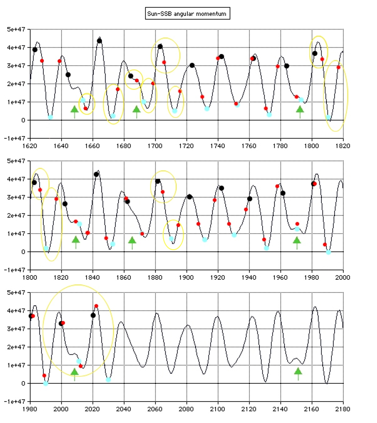
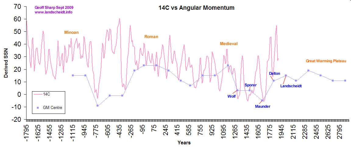
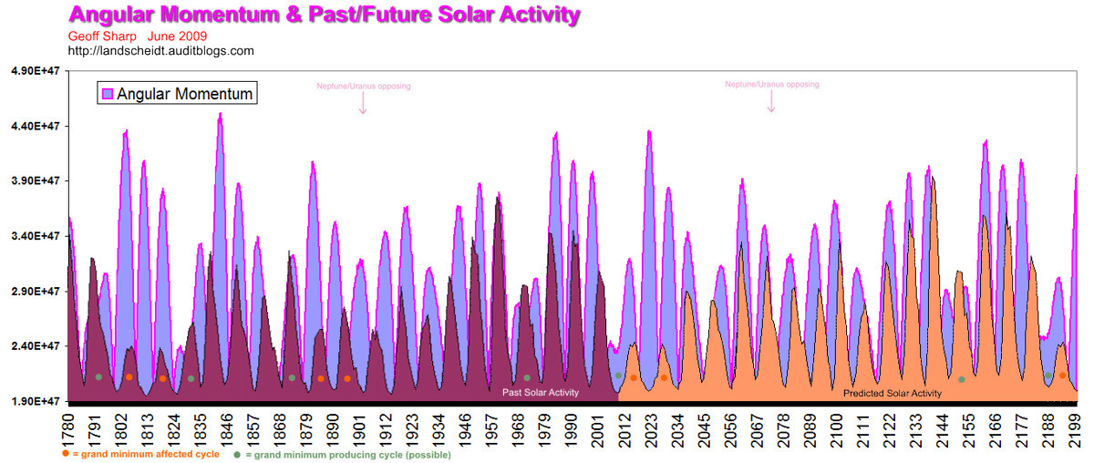
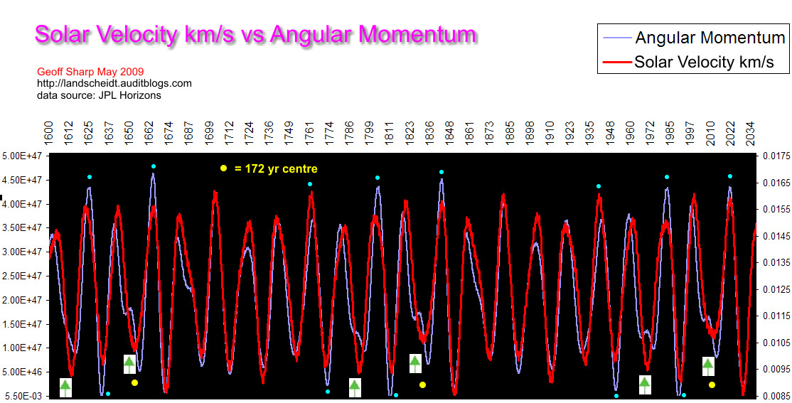
Solar Angular Momentum graph produced by the late Carl Smith 2007. Annotations and green arrows added.

Planetary influence over solar cycle output and solar grand minima has been theorized since the early days of Rudolf Wolf.  Jose was the first to gain traction in 1965 and was then followed by major players Landscheidt, Fairbridge and Charvàtovà who published many papers but were never really taken seriously by the scientific public at large. All the aforementioned authors have made solid contributions to this valuable area of research and without this base knowledge I am sure the late Carl Smith would never have had the motivation to produce his soon to be famous (I believe) solar angular momentum graph (2007).

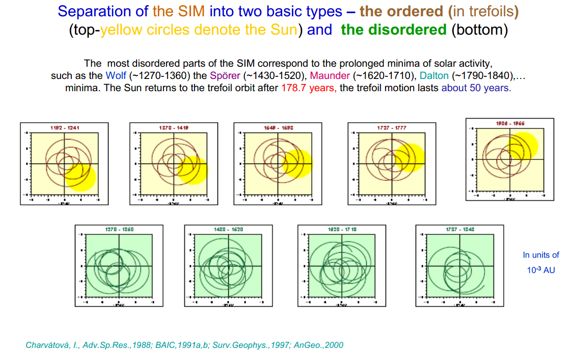
In my opinion Charvàtovà had the most to offer where she picked up on the Jose SIM diagram that displayed the irregular orbit pattern of the Sun around the solar system barycentre (SSB). She noticed that during times of grand minima the orbit pattern changed which is a major break through and now with the added data from Carl we can now understand and quantify this change, but more on that later.

Jose believed there was a recurring 179 year pattern that controlled the Suns orbital path around the SSB, this was the original discovery that recognized the returning SIM pattern that controls our Sun. While he was in the ballpark we now know through Carl’s graph and JPL data that this pattern is indeed very loose but none the less there is a recurring occurrence of grand minima over the Holocene that centres around the synodic period of Uranus and Neptune (171.4 years) but this can only be used as a rough guide and is not capable of predicting grand minima down to the solar cycle like we can today.

Landscheidt wrote many papers and a book which covered planetary harmonics and their interconnection with solar and Earth functions which included ENSO, atmospheric teleconnections, lake levels, fish and animal populations as well as the stock market. His most famous prediction was for a solar grand minimum between 1990 and 2070 which would peak at 2030 in his book Sun-Earth-Man (1989). Landscheidt used one single dataset to produce this forecast which follows the solar torque readings that result from the changing solar orbit shape directly influenced by the planet positions. Once again he was in the ball park but I believe through Carl’s graph we can now drill down much further to reveal a far higher level of accuracy when looking at each solar cycle, when we do this Landscheidt’s predictions I think will prove to be out of place. Below are two graphs that Landscheidt used to form his prediction.

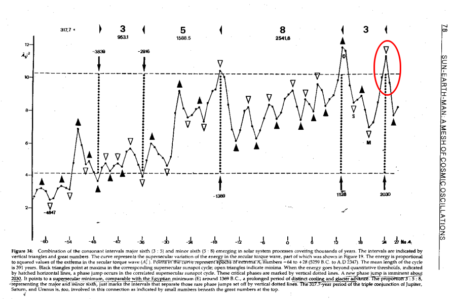
Taken form Sun-Earth-Man pg 78 showing the torque curve that Landscheidt used for his prediction. The Landscheidt torque curves vary wildly from the standard AM curves. Note there is no torque extrema during the Little Ice Age. Click for a larger view.

The following is the excerpt from his book where his prediction is first noted.

“When subsets are  formed,  the results  prove  to be homogeneous.  The torque wave
points  to  a  secular sunspot  minimum past 1990.
The  extrema in  the  secular  wave of  IOT  can  be taken to constitute  a  smoothed
supersecular wave with  a  quasi-period of 391  years.  This  long wave points to
an  imminent  supersecular  sunspot  minimum  about 2030.  There  are
indications  that  secular  and  supersecular  sunspot  minima are  related  to
variations in  climate. Thus a  prolonged period of  colder climate is about to be
initiated  by the  secular minimum past  1990, will reach its  deepest point around
the  supersecular minimum  in 2030, and  come to an end  about 2070. “

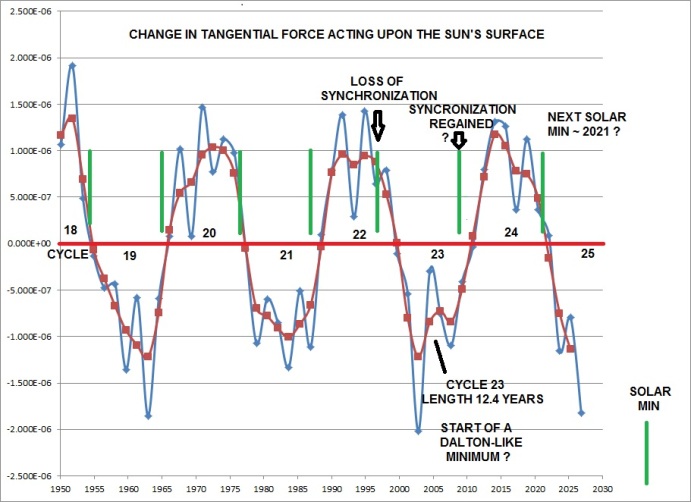
In a later paper Landscheidt uses a different torque graph to reinforce his 2030 prediction but now moves away from the 1990 prediction which of course did not occur. The following is taken from a comment I published 3 years ago on this site.

Here is the original graph that Landscheidt used in his predicted 1990 and 2030 grand minimum. The red dots highlighting those years. Also included is his original text showing his reasoning. The level of detail between his data and Carl’s is many orders different, but you can see the general trend in the past followed roughly by grand minima. When the AM or torque dips below the dotted line there is a solar slowdown, but he is just picking up markers that occur around the same time and not seeing the actual driver. Note that Landscheidt predicts this grand minimum to be of a similar strength and timing as the Maunder….I wonder what he would think now, if he were still with us today?

Fig. 11:Time series of the unsmoothed extrema in the change of the sun’s orbital rotary force dt for the years 1000 – 2250. Each time when the amplitude of a negative extremum goes below a low threshold, indicated by a dashed horizontal line, a period of exceptionally weak solar activity is observed. Two consecutive negative extrema transgressing the threshold indicate grand minima like the Maunder minimum (around 1670), the Spoerer  minimum (around 1490), the Wolf minimum (around 1320), and the Norman minimum (around 1010), whereas a single extremum below the threshold goes along with events of the Dalton minimum type (around 1810 and 1170) not as severe as grand minima. So the Gleissberg minima around 2030 and 2200 should be of the Maunder minimum type. As climate is closely linked to the sun’s activity, conditions around 2030 and 2200 should approach those of the nadir of the Little Ice Age around 1670. As explained in the text, the IPCC’s hypothesis of man-made global warming is not in the way of this forecast exclusively based on the sun’s eruptional activity. Outstanding positive extrema have a similar function as to exceptionally warm periods like the Medieval Optimum and the modern warm period.

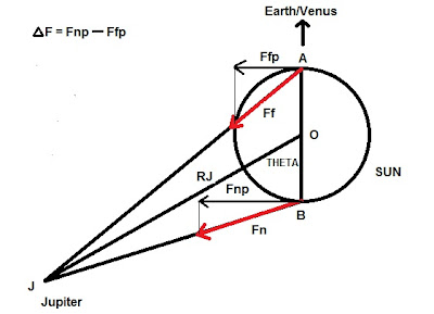
Landscheidt is using torque extrema that occur when Saturn/Uranus and Neptune line up with Jupiter opposing. During this event the Sun returns very close to the SSB (red crosshairs).

This is where the Landscheidt marker is close to where grand minima occur but unfortunately is very vague. The marker can only occur near a Uranus/Neptune conjunction which is also what is required to trigger the angular momentum perturbations (AMP event) shown via the green arrows in Carl’s graph, but the conjunction can be decades away from the AMP event and can produce erroneous predictions. The current event should be short and weak like the Dalton Minimum and the 2200 event will also be weak if we follow Carl’s graph which has successfully predicted the current grand minimum and hindcast grand minima throughout the Holocene.

Solar cycle prediction based on angular momentum (AM). AM is important for overall cycle strength and solar grand minima.

There is much research on the AMP events on this website and I suggest a good place to start is the “Published Paper” link at the head of this site.

Further evidence of Landscheidt’s prediction of a 1990 solar grand minimum is observed in his 1981 paper “Swinging Sun, 79-Year Cycle, and Climatic Change” where he states;

“As to practice, it seems possible now to calculate the date, the phase, and the amplitude of long-term solar variations in past and future. It is no longer necessary to recur to ultralong cycles with a duration of hundreds or thousands of years. The irregular distribution of the rare impulses of the torque of great strength offers a simpler explanation of ultralong-term variations. Fig. 4 shows the future course of the 79 YC. The next negative RDM will be released in 1990. It meets the criterion Cn2. The amplitude can be assessed by the Sit-value which is equal to| 4.23| U. The minimum about 1811 reached only 2It =| 4.07| U. Relatively small differences in the 2It-data lead to relatively great differences in the amplitudes. This can be seen from Table 2. Thus it may be expected that the negative RDM 1990 will be distinctly more pronounced than the 1811-minimum……..It is to be expected that the climatic conditions in at least three decades after 1990 will be more severe than after 1811 as corresponds to the ratio 2 lt = |4.071 U(RDM 1811) toSlt =|4.23| U (RDM 1990) compared with 2 |t = l 4.43| U (RDM 1671)”

Of interest Fairbanks predicted a 1990 solar grand minimum using the same zero crossing method and Jose cycle as Landscheidt. Below is an excerpt from Fairbridge’s 1987 paper.

I think it is pretty clear that although Landscheidt and Fairbridge are on the right track their failed predictions show there is something missing in their base theory. It is also interesting that Landscheidt did have similar data that is presented in Carl’s graph but he failed to recognize the significance. In his 1989 book on pg 16 he states:

“As has  been shown  already,  the Sun’s surface is  a boundary in terms  of  the
morphology of  nonlinear  dynamic  systems.  Thus,  it  makes  sense  that  the
major instability  events starting about  1789,  1823,  and  1867, and  later about
1933 and  1968, occurred  just  when the centre of  mass remained in or near  the
Sun’s  surface for several years.
When the Sun approaches the centre  of  mass (CM),  or recedes from it, there
is  a phase when CM  passes through  the Sun’s  surface. Usually, this is  a  fast
passage,  as the  line  of  motion is  steeply inclined  to the  surface. There  are  rare
instances,  however, when the  inclination  IS  very  weak,  CM  runs nearly
parallel with the Sun’s  surface,  or oscillates  about  it  so that  CM  remains  near
the  surface for several years.  Fixing  the  epochs of  start and end of  such periods
involves  some  arbitrariness.  The  following  definition is in  accordance with
observation  and  meets all requirements  of  practice:  major solar  instability
events  occur  when the centre  of  mass remains continually within the  range
0.9 –  1.1 solar radii  for  2.5 to 8.5 years,  and  additionally within the  range  0.8
–  1.2  solar radii for  5.5 to  10 years.  The  giant planet  Jupiter is  again involved.
In most cases major instability events  are released  when Jupiter is stationary
near CM.
The  first, sharper criterion yields the  following periods:
1789.7 –  1793.1  (3.4  yr)
1823.6 –  1828.4  (4.8  yr)
1867.6 –  1870.2  (2.6  yr)
1933.8 –  1937.3  (3.5  yr)
1968.4 –  1972.6  (4.2  yr)
2002.8  –  2011.0  (8.3  yr)
The  first decimal is  only given to relate  the results rather  exactly  to the  aiterion.
The  epochs of  the onset  and  the  end  of  the  phenomenon  cannot  be assessed
with such precision. The  second, weaker criterion yields periods which begin
earlier:

1784.7 –  1794.0  (9.3 yr)
1823.0 –  1832.8  (9.8  yr)
1864.5  –  1870.9  (6.4 yr)
1932.5 –  2938.3  (5.8 yr)
1967.3 –  1973.3  (6.0  yr)
2002.2 –  2011.8  (9.6  yr)
Henceforth,  the  starting  periods  1789,  1823  etc.  of  the  first  criterion  will  be
quoted.
In case  of  major instability  events  that  affect  the  Sun’s  surface and  the
incidence of  features  of  solar activity displaying in this  thin, sensitive layer
the  instability seems  to spread out in the  planetary system and seize  all events
in time series that are  connected with the  Sun’s activity.”

When Landscheidt talks of major instability events he is NOT referring to solar output, but instead he is using this event as a place in time where phase reversals occur. ie where he uses the minima instead of maxima of extrema in the particular dataset he is employing. The major instability events according to Landscheidt affect rise and fall of animal populations, economic turning points, stock prices, interest rates, global periods of general instability and even human creativity. Landscheidt in later papers moves away from these less than scientific statements but at no point associates these events with reduced solar output.

And in another graph I highlighted 3 years ago:

I found another graph that Landscheidt uses in “Solar Eruptions Linked to North Atlantic Oscillations” that shows that he DID have access to information at a more precise level. Here he shows the “camel humps” like we see in Carl’s AM graph but this graph is based on torque measurements (which are similar to AM). Landscheidt calls these perturbations PTC (perturbed torque curve) and he states that they occur every 35.8 years, and are responsible for “phase reversals”. My research and Carl’s suggest the PTC type disturbance does not occur on a repeating pattern, but only when Neptune & Uranus are in or near conjunction. This I think is further evidence that Landschiedt perhaps missed this vital piece of the puzzle???? 

Landscheidt used many planetary cycles to compare with solar and earth cycles. In particular he employed the alignment between the Sun/SSB and Jupiter. What he found was that the correlations went out of phase over time but invoked a phase reversal so that he could use both minima and maxima of a given cycle. He uses the PTC event (major stability event) which is the same as the green arrows on Carl’s graph as a position for phase reversal but completely misses that these events are what correlate with all solar slowdowns and the altered solar path that Charvàtovà made her name on. He incredibly was so close, but unfortunately no cigar.

In a recent article Roger Tattersall (tallbloke’s talkshop) on his blog that is predominately focused on planetary theory makes the mistake of stating that Landschiedt uses the PTC type or major instability events to predict solar slowdowns, this is obviously incorrect. I have tried to inform him of his error but to date he is reluctant to change his incorrect and misleading views.

This is where we pick up on Charvàtovà. In the 1988 she produced a paper “The Relations Between Solar Motion and Solar Variability” showing that grand minima occur when the solar orbit is disordered over longer periods. All past grand minima have shown a correlation with this disordered pattern about the SSB so she is definitely on the ball but sadly does not continue her research into the ultimate reasons for the disordered orbit. She hints that the conjunction of Uranus and Neptune are at the centre of grand minima epochs like Landscheidt but fails to drill down to the underlying causes or how each disordered orbit can be quantified in relation to the strength of a solar slowdown.

In 1988 she predicts a period of lower sunspot activity and longer cycles from 2000-2030 and the epoch will be more Dalton like which is more accurate than Landscheidt (if my predictions pan out) but she does not see the planet position of Jupiter/Uranus/Neptune with Saturn opposing that individually creates the disordered solar pattern. Her later papers and slide shows also display this omission. Her 2000 paper describes a period of disordered orbit from 1985-2030 but she missed the disordered orbit at 1970 which coincides with the low solar cycle SC20.

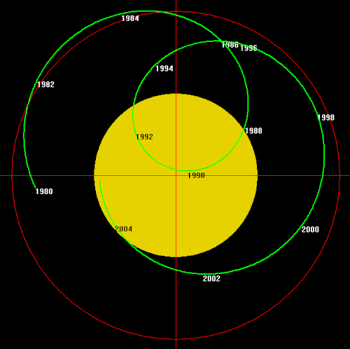
The above planet sequence is the main driver of the disordered pattern that happens either side of the U/N conjunction. Below is an image of how the solar orbit varies (purple line)

The green arrows on Carl’s graph align with the above planetary position and the altered purple orbit path. The main disruption only occurs during the inner loop but looking at the shape of the loop alone does not give enough detail to distinguish a low cycle from a grand minimum type cycle. The altered path of 1970 does not look all that different to the current path but there should be quite some difference between SC20 and SC24 in terms of solar output. This is where Carl’s graph comes in and we can quantify the AMP event that happens at the green arrows. I have tried to contact Dr. Charvàtovà without success, but I am sure she would be interested to see the relevance of Carl’s graph in relation to her work.

Carl was not aware of his discovery when he created the graph and sadly when I pointed it out to him he was happy but had other matters on his mind, as you would expect when suffering from terminal cancer. Carl rewarded me by passing on his blog to me and Carl’s brother David has sponsored me in the hope of furthering Carl’s work. I consider myself lucky to have stumbled on Carl’s graph which I will endeavour to push as the rosetta stone of solar science.

Unfortunately todate no one in the science arena has picked up on this discovery which was first published online in 2008, the topic is banned at WUWT (the largest science forum on the web) and so far has been largely ignored by planetary forums including Tallbloke’s Talkshop. Hopefully this will change in the future when the large amount of information is gradually absorbed and the predicted solar grand minimum takes hold.

Grand Harmonic Climate Model

Solar system dynamics are interwoven into all aspects of life as we know it. Gravity being the ultimate blacksmith that shapes our destiny. The very driver of the Sun’s Dynamo and Earth’s climate are harmonic resonances between the larger bodies in our solar system, which also mesh with magnetic/electrical forces.

These harmonic drivers can be broken down to three levels.

1. The Ice Age Cycles (Milankovitch, 100,000 years)(J/S/U/N)

2. Solar Grand Minimum & Solar Modulation Cycle (Sharp, 172 years)(J/S/U/N)

3. PDO/ENSO Harmonic Cycle (Scafetta, 60 years)(J/S)

This article will deal with the brief concepts behind each of the 3 levels along with interaction of each level with our atmosphere and,  how each player is inextricably linked with all layers of the atmosphere that work together to form a complex organic total system.

Level 1 was first proposed by Milutin Milankovitch during the years of the first world war. Planetary gravity forces from the outer 4 planets over 100,000 years gradually change the shape of Earth’s orbit from circular,  to elliptical along with shorter term changes in the inclination angle and winter precession timing. When a particular combination of the orbital elements is reached, high latitudes of the northern hemisphere begin to experience year round snow. This triggers year on year ice growth because of albedo changes, that now reflect solar energy away from Earth. The Earth spends 90% of its time in frozen conditions, with the recent warm Holocene period (11,500 yrs) drawing to an end. Ice Age cycles once invoked, over ride the smaller influences of level 2 and 3.

During the warmer Holocene type periods level 2 & 3 harmonic cycles rule the day.

Level 2 was outlined in rough terms by pioneers such as Jose, Landscheidt and Charvàtovà who each identified crucial components, which where brought together and quantified with the assistance of Carl Smiths solar angular momentum graph. The new information led to discoveries which enabled quantification of the precise timing and strength of past and future solar grand minima, along with the discovery of the 172 year solar powerwave. This wave controls the overall solar cycle modulation. Many references can be found on this site on level 2 theory, along with a published paper found HERE. A recent paper by Wolff and Patrone (2010) has provided a physical mechanism for angular momentum theory. In summary level 2 forces shape the Holocene solar output and Earth temperature overall trends.

Level 3 is a well known 60 year cycle in Earth’s temperature record that in recent times aligns with the PDO/ENSO record. Nicola Scafetta has documented in several papers how the temperature record coincides with two solar system harmonic patterns. The solar velocity 60 year cycle and the Jupiter/Saturn synodic harmonic cycle along with Lunar harmonics being the thrust of his proposals. Level 3 influences can be strong, and potentially over ride level 2 when the 2nd level is not in a deep low stage. Level 2 is always present,  but having different influences depending on timing. The 60 year cycle in Earth’s temperature is most likely controlled by the PDO index which over the last 100 years aligns with global temperature. The PDO index is often portrayed by the warmist crowd as an “after effect of ENSO” in some attempt to diminish the crucial role the PDO plays in climate fluctuation, preferring us to believe CO2 is the main driver. In 2011 we saw clear evidence of the warm pool in the Pacific northwest (which is the main characteristic of the cool PDO phase) IS capable of “charging” the Walker Circulation pump that drives La Nina and inhibits El Nino. The neg PDO warm pool was responsible for the last stage of the back to back La Nina of 2010/11. The presence of the 30 year PDO warm pool will tend to favour La Nina over El Nino events which regulates Earth’s climate.

Further research is required to determine the cause of the PDO, but I am backing Dr. Scafetta at this point.

Effects on Earth’s Atmosphere.

Earth’s atmosphere may be broken up into multiple layers but each layer is part of a functioning overall system. The troposphere where we live (0-10km) is very much interlinked with all the layers above. Each layer receives different influences from the energy sources available, but interrelate as a whole, to form weather patterns experienced on the surface. When it comes to level 2 energies, the most variable are solar UV outputs, which have large potential to alter climate cycles.

Solar UV ranges from 10-400nm on the spectral scale and is broken up into 3 basic categories. EUV is at the extreme end of the spectrum (10-125.6nm) which includes the important Lyman alpha portion which resides at the high end of the EUV scale. EUV values vary by 30-100% across the range over the solar cycle, and have the most potential to modulate atmospheric chemistry, size and temperature. FUV (126-200nm) also shows big variations in the 10-30% range and is a very important player along with EUV for ozone formation in the stratosphere and mesosphere. MUV (200-300nm) is a solid ozone backstop but only varies 1% over the solar cycle but still relevant when comparing overall TSI (total solar irradiance) variance of 0.1%.

Those that subscribe to the AGW religion will only push TSI when it comes to solar influence on climate. The records gathered from somewhat dubious satellites during the space age display a small 0.1% change in solar HEAT output over a few solar cycles. To really appreciate the true solar effect on climate it is necessary to include chemical changes and total solar influenced cloud cover to see the real picture.

Beginning with the most variable component of solar output spectrum, EUV has only in the last few decades been studied in detail, and is now one of the areas where real dollars are spent in space exploration.

EUV is mainly consumed above 100km in the thermosphere where the air density is low. Some of the climate relevant reactions occur in this region producing atomic oxygen and nitric oxide that later play a large role in ozone formation/control at lower levels. In the EUV range there is an important lively band in the Lyman alpha range (125.6nm) that penetrates down to 70km. As seen in the above diagram different ranges of the UV spectrum are absorbed at different altitudes, the Lyman alpha range is particularly strong and produces large amounts of atomic oxygen down to 70km that is used in the formation of ozone in the mesosphere. Soloman (1982) and others show how this atomic oxygen is also pumped down to lower levels to further assist ozone production, the downward mechanism coming from eddy diffusion. EUV can produce species that build ozone but it can also produce large quantities of nitric oxide (NO), that destroys ozone. Nearly all NO is produced in the thermosphere, with the majority portion coming from EUV interaction. But, during times of high aurora activity a process called EPP (Energetic Particle Precipitation) can produce as much as 50% of the total NO production. Solar proton events and cosmic rays also play their part which all come under the general umbrella of solar modulation. Several authors including (Soloman, 1982) and a good overall reference HERE  have shown that great quantities of NO are diffused down to the mesosphere and stratosphere where they have great influence in ozone formation (negative). The downward path coming from eddy diffusion and the downward flow to the northern polar vortex at the tale end of planetary and gravity waves. The ozone process is complex and little understood, but recent finds by Haigh are showing quantities of ozone can increase above 45km and decrease below during times of weak solar activity, which is no doubt brought about by the chemical changes that fluctuating EUV/FUV brings along.

Baldwin et al who are considered the experts in the QBO (stratospheric wind oscillation) speculate on the role of UV in the mesosphere and how modulation could play an important role in the break up of the northern polar vortex. The break down of the vortex is a key component of the AO index which is hard linked to the behavior of the jet stream.

“Because of the strong absorption of ozone in the UV occurring in the upper stratosphere and meso-
sphere, a solar influence on the thermal structure in these regions of the atmosphere is plausible. This, in
turn, might affect the strength of the planetary wave driven “extratropical pump” [Holton et al., 1995]. A
mechanism involving downward propagation of stratospheric anomalies, through modification of planetary
wave propagation from below, is discussed in section 6.2.”

The jet stream changes which drive cold air from the polar regions has provided colder conditions for the past 3 years, any changes to cloud cover extent which is also proposed by harmonic drivers will further increase the influence from exterior sources.

The links between solar activity and climate remain controversial, but headway is being made to oppose the IPCC rhetoric and dogma. Similarly the planetary links to solar and PDO drivers are also making headway as more research comes to hand. Nicola Scafetta has already proposed a Harmonic Climate Model which deals with the level 3 oscillations. Nicola is very aware of the higher levels that need to be fully incorporated, which perhaps may happen in print in the not too distant future.

Scafetta’s New Paper Linking Mid-Latitude Aurora to the 60 Year Temperature Cycle.

Nicola Scafetta has just sent me a copy of his latest paper “A shared frequency set between the historical mid-latitude aurora records and the global surface temperature”

http://www.sciencedirect.com/science/article/pii/S1364682611002872

The abstract follows:

Herein we show that the historical records of mid-latitude auroras from 1700
to 1966 present oscillations with periods of about 9, 10–11, 20–21, 30 and
60 years. The same frequencies are found in proxy and instrumental global
surface temperature records since 1650 and 1850, respectively, and in
several planetary and solar records. We argue that the aurora records reveal
a physical link between climate change and astronomical oscillations. Likely
in addition to a Soli-Lunar tidal effect, there exists a planetary
modulation of the heliosphere, of the cosmic ray flux reaching the Earth
and/or of the electric properties of the ionosphere. The latter, in turn,
has the potentiality of modulating the global cloud cover that ultimately
drives the climate oscillations through albedo oscillations. In particular,
a quasi-60-year large cycle is quite evident since 1650 in all climate and
astronomical records herein studied, which also include a historical record
of meteorite fall in China from 619 to 1943. These findings support the
thesis that climate oscillations have an astronomical origin. We show that a
harmonic constituent model based on the major astronomical frequencies
revealed in the aurora records and deduced from the natural gravitational
oscillations of the solar system is able to forecast with a reasonable
accuracy the decadal and multidecadal temperature oscillations from 1950 to
2010 using the temperature data before 1950, and vice versa. The existence
of a natural 60-year cyclical modulation of the global surface temperature
induced by astronomical mechanisms, by alone, would imply that at least
60–70% of the warming observed since 1970 has been naturally induced.
Moreover, the climate may stay approximately stable during the next decades
because the 60-year cycle has entered in its cooling phase.

Dr. Scafetta has written several papers on the 60 year trend in global temperatures that align with a 60 year trend in the Solar velocity records. This same trend aligns with PDO record which is a warm and cool phase of the Pacific Ocean that also aligns with the frequency in the ENSO cycle (whether La Nina or El Nino’s dominate). This new paper demonstrates a 60 year period in the mid latitude auroras that suggests a solar output astronomical link in the 60 year cycle.

The theory suggests that during times of low solar output the reduced solar wind allows more cosmic rays to excite the outer atmosphere which then enhance any solar flare activity to a state whereby aurora can be visible at mid latitudes. The 266 year history for the most part does look to show a 60 year fluctuation with perhaps an irregularity around 1950-60. I am not totally convinced with this logic as mid latitude aurora can be a function of an over active Sun also which is in competition. (note: my initial reading of the paper was incorrect, see update below)

The possible causes of the PDO are of immense importance to understanding what drives the world climate and while I am not convinced with the aurora argument (see update) Dr. Scafetta does produce another interesting graph that corresponds very closely with the PDO record.

Graph A above displays the tidal effects on Earth from Jupiter & Saturn. A very clear 60 year period is observed which closely aligns with Graph B from his earlier papers that show the modulation of solar velocity. The two forces may be related but are quite distinct from one another. Solar velocity is modulated by the distance the Sun travels away from the SSB (solar system barycentre). The further the distance the faster the Sun travels around the SSB which is totally modulated by Uranus and Neptune. During my research I found the 60 year period came about from the positions of Uranus and Neptune during the Jupiter/Saturn conjunction/opposition. When Uranus/Neptune are together they provide boost (distance) to the Sun and also at other times when either Uranus or Neptune come together with the Jupiter/Saturn conjunction causing a triple conjunction. The last few hundred years shows this 60 year trend in solar velocity but I suspect that might change over longer periods.

Graph A is completely different and shows tidal effects on earth that are not subject to planetary precessions and is far more accurate in my opinion of maintaining a more precise longer lasting 60 year period. The synodic period of Jupiter and Saturn does not vary with planet precession although their perihelion positions will vary over time producing a minor change. In April 2009 I produced a graph that nearly mirrors Nicola’s graph A but is based on the Jupiter perihelion/aphelion distances.

The modulation in Jupiter’s perihelion/aphelion distances is mainly brought about in my opinion by the gravitational perturbations induced by Saturn, a link to my original research can be found HERE. I am at odds with many in the scientific community that believe the gas giants do not orbit the Sun. Most I have had discussions with are of the opinion that the outer planets orbit the SSB, but my research strongly suggests at least Jupiter and Saturn have the Sun as their orbit axis point. Whether  the Jupiter distance is controlled by planet perturbations or a moving Sun away from the planet axis point there is a modulation of 60 years in the Jupiter perihelion distance that looks to align with the PDO record. Could Jupiter tidal effects somehow control the PDO state? Without a driver we are still in the dark.

Past research on the planet orbit axis points can be found HERE and HERE.

UPDATE: Nov 10 2011.

Dr. Scafetta has pointed out to me that I missed the main point of the mid-latitude aurora driving force. While mid latitude aurora can be a function of increased solar output, the Earth’s magnetosphere could be affected by planetary influence in isolation that could have downstream effects on cloud cover. Dr. Scafetta has reported on the quasi 60 year cycle of mid-latitude aurora that corresponds with the Jupiter/Saturn tidal measurements very accurately, but leaves the physical mechanism responsible to others that might like to research further.

On reading the paper there are several references to a planetary influence on the Earth’s magnetosphere and how increased cosmic flux excites the outer atmosphere leading ultimately to more mid-latitude auroras (and changes in cloud cover). My reading being from a solar/planetary background was that the planets were affecting solar output thereby influencing the solar wind and ultimately affecting our magnetosphere and cosmic flux levels received. This is not the thrust of Dr. Scafetta’s paper which points out a possible planetary effect directly on our magnetosphere. This in my opinion greatly changes the magnitude of what I think is a very important enlightening new paper.

Some extracts from the paper.

Thus, the declination measures the direction of the gravitational and magnetic forces of Jupiter and
Saturn relative to the daily average orientation of the terrestrial magnetosphere.

This returning pattern gives origin to a quasi-60-year physical
tidal cycle on the Sun and in the heliosphere in proximity of the
Earth’s orbit. A similar quasi-60-year periodic pattern would be
generated by the magnetic fields of Jupiter and Saturn that influence
the heliosphere too.

Fig. 9 summarizes a chain of mechanisms that, according to
the finding of this paper, reasonably links the planetary motion to
climate change through solar and heliosphere modulation of the
magnetosphere and ionosphere that regulate the cloud cover
percentage.

It is possible that when Jupiter and Saturn are closer to the Sun,
there may be an increased solar activity because of the stronger
planetary tides and other mechanisms (Wolff and Patrone, 2010),
and a stronger magnetic field within the inner region of the solar
system forms, although the patterns may be more complicated
because of the presence of other cycles that will be discussed in
another paper. A stronger solar or heliospheric magnetic field better
screens galactic cosmic ray fluxes. Fewer cosmic rays reaching the
Earth imply a weaker ionization of the upper atmosphere. As a side-
effect, less auroras form in the middle latitudes because a stronger
magnetic field and a less ionized ionosphere mostly constrains the
auroras in the polar region. In addition, the level of ionization of the
atmosphere has been proposed as an important mechanism that can
modulate the low cloud cover formation (Tinsley, 2008; Kirkby,
2007; Svensmark et al., 2009). Essentially, when the ionization is
weaker, less clouds form. In conclusion, a solar and heliospheric
modulation of the cloud system would greatly contribute to climate
change through an albedo modulation (see Eq. (8)).

Also of interest is the value of using the quasi 60 year aurora/planetary data to forecast future global climate. Below is two graphs from the paper doing just that. The physical mechanism is not required for forecasting if the hindcasting is strong and the planetary future positions are known.

Below is some of the email text from Dr. Scafetta which may serve to explain some of the detail.

What the paper does is to show that the mid-latitude aurora records present the same oscillations of the climate system and of well-identified astronomical cycles. Thus, the origin of the climatic oscillations is astronomical what ever the mechanisms might be.

In the paper I argue that the record of this kind of aurora can be considered a proxy for the electric properties of the atmosphere which then influence the cloud cover and the albedo and, consequently, causes similar cycles in the surface temperature.

Note that aurora may form at middle latitude or if the magnetosphere is weak, so it is not able to efficiently deviate the solar wind, or if the solar explosions (solar flare etc) are particularly energetic, so they break in by force.

During the solar cycle maxima the magnetosphere gets stronger so the aurora should be pushed toward the poles. However, during the solar maxima a lot of solar flares and highly energetic  solar explosions occurs. As a consequence you see an increased number of mid-latitude auroras despite the fact that   the magnetosphere is stronger and should push them toward the poles.

On the contrary, when the magnetosphere gets weaker on a multidecadal scale, the mid-latitude aurora forms more likely, and you may see some mid-latitude auroras even during the solar minima as Figure 2 shows.

In the paper I argue that what changes the climate is not the auroras per se but the strength of the magnetosphere that regulates the cosmic ray incoming flux which regulate the clouds.

The strength of the magnetosphere is regulated by the sun (whose activity changes in synchrony with the planets), but perhaps the strength of the Earth’s magnetosphere is also regulated directly by the gravitational/magnetic forces of Jupiter and Saturn and the other planets whose gravitational/magnetic tides may stretch or compress the Earth’s magnetosphere in some way making it easier or more difficult for the Earth’s magnetosphere to deviate the cosmic ray.

So, when Jupiter and Saturn get closer to the Sun, they do the following things: 1) may make the sun more active; 2) the more active sun makes the magnetosphere stronger; 3) Jupiter and Saturn contribute with their magnetic fiend to make stronger the magnetic field of the inner part of the solar system; 4) the Earth’ magnetosphere is made stronger and larger by both the increased solar activity and the gravitational and magnetic stretching of it caused by the Jupiter and Saturn. Consequently less cosmic ray arrive on the Earth and less cloud form and there is an heating of the climate.

However, explaining in details the above mechanisms is not the topic of the paper which is limited to prove that such kind of mechanisms exist because revealed by the auroras’s behavior.

The good news is that even if we do not know the physical nature of these mechanisms, climate may be in part forecast in the same way as the tides are currently forecast by using geometrical astronomical considerations as I show in Figure 11.

I am particularly excited that this paper perhaps gives us some insight into the workings of the PDO which I think is the main driver of the global climate system. It may be possible that planetary influence on our magnetosphere influences cloud cover that could determine the spatial SST values that control the PDO, this indeed could be a very big step in our understanding of the climate system.

A copy of the complete paper can be found HERE.

Solar Cycle Induced by Rotating Medium.

Bart Leplae has a new paper published in the General Science Journal that proposes a new method of spin orbit coupling that could be responsible for rotation changes at the Sun. Bart outlines a few principles in his introduction.

Introduction
• Scientific Publication: “Does a Spin–Orbit Coupling Between
the Sun and the Jovian Planets Govern the Solar Cycle?”
(I. R. G. Wilson, B. D. Carter, and I. A. Waite, 2007):
– Presents evidence to show that changes in the Sun’s equatorial
rotation rate are synchronized with changes in its orbital motion
about the barycentre of the Solar System
– Proposes that this synchronization is indicative of a spin–orbit
coupling mechanism operating between the Jovian planets and
the Sun
– While data are consistent with the idea that there is a spin–orbit
coupling between Jupiter and the Sun, it does not tell anything
about the true nature of the underlying mechanism that might
be causing this coupling
• This paper proposes the Rotating Medium Model as the
underlying mechanism for the Spin-Orbit Coupling.

A link for the paper can be found at   http://www.wbabin.net/files/4354_leplae4.pdf

The paper does not explain how planetary alignment might affect solar rotation rates during solar grand minima but other points might be of interest to readers. Comments and discussion is encouraged.

Is the World Ready for another Ice age?

Little Ice Age conditions are sweeping across most of the northern hemisphere creating travel chaos, financial damage and, unfortunately, many deaths in the process. I predicted this back in July 2010 in my “ A Massive Winter Heading for the Northern Hemisphere?” article that has come home to roost. An excerpt  “I predict the extra boost from my predicted solar grand minimum along with the current oceanic conditions the next northern winter will experience conditions similar to the Little Ice Age (1250-1850).”

The conditions are perfect at present for continued cold, the oceans are cold with the important atmospheric oscillations forcing cold arctic air further south than usual. The negative AO and NAO are producing blocking high pressure cells that bend the jet stream which allows the southern movement of arctic air. At present there is an unusual permanent high pressure cell over Greenland.  I think this pattern should prevail over the next 20 to 30 years and replaces the positive pattern of the last 30 years. The global warming models have suggested that man-made CO2 will keep the AO and NAO in positive mode….how wrong have they been?

Many are asking what causes the global ocean and atmospheric oscillations to follow these heating and cooling trends. The Pacific Decadal Oscillation (PDO) is a large player that has a 60 year cycle, this follows the solar velocity oscillations as the sun orbits the centre of the solar system as described by Scafetta. The NAO works very closely with the PDO but is possibly governed by changes in the height of the atmosphere as a result of the reduced EUV that is a product of a quiet Sun. NASA has reported that the height of the Thermosphere is at the lowest point since records began; EUV is a controller of atmospheric height. We are told that the TSI or total heat output of the Sun only varies by 0.1 percent over a typical solar cycle. But we are now learning that the Sun has other ways of affecting climate that the models have not allowed for. EUV is capable of a 16% (correction: 30-100% depending on wave length) modulation over the cycle and, at present, is refusing to ramp up. This current minimum sees the EUV level 15% lower than the previous minimum which, if correct, dispels the theory of a solar base floor.

With solar output being so crucial to climate, where are we heading in the next hundred years?

Right now I think we are heading into a solar grand minimum that will last 2 cycles producing a very different world compared to what we have experienced over the last 30 years. After that a brief warming will occur before slipping into a familiar pattern that started in the early 1900’s, which is more cooling gradually warming over several decades. The Sun is controlled by its angular momentum which is in turn controlled by the outer planets…My published paper has all the details for those wishing to dig deeper.

Click on the pic for a larger view.

But is there more? There are two types of global cooling – one is solar output modulation as discussed, but lets look at the other. Over the past several million years the planet has spent around 80% of its time under ice. There is a regular pattern as discovered in the Vostok ice cores that show us a roughly 100,000 year cycle of ice ages. Mankind for the past 11,000 years has enjoyed the Holocene which is an interglacial or warm period that will soon come to an end. The outer planets over long periods influence the shape of the earth’s orbit via gravitation perturbations. This has the effect of changing the way heat is received from the Sun which leads to a gradual build up of snow/ice that does not melt during summer in the northern hemisphere. But looking at the ice core records we can see a fairly abrupt change in temperature that suggests there is another factor in play governing what tips us into the ice age plunge. It is very possible that a solar grand minimum that is in position at the right time could assist the natural orbital changes as outlined via the Milankovitch Cycles. A kick start forced on by 30 years of negative PDO, AO and NAO might be all that is needed to push us over the edge…we are well overdue, but of course this is highly speculative.

We are now two years into solar cycle 24 and today we are heading into our 8th consecutive spotless day as counted by the Layman’s Count.  This cycle is currently undercutting the first cycle of the Dalton Minimum. Solar F10.7 flux has struggled to get over 80 all year and currently this month is likely to show a further decline. If you would like to follow the daily progress of solar cycle 24 be sure to check out the Layman’s page and I also encourage any questions and discussions relating to this article, simply register as a user and fire away.

New Evidence of Barycentric Motion of Exoplanet Host Stars.

A new paper by Perryman M.A.C. & Schulze-Hartung T. has been published on the 5th October 2010 that records the barycentric motion of distant stars that have exoplanets.

A link to the full paper found HERE.

Barcentric movement is a principle component of discovering exoplanets belonging to distant stars which display a wobble over time. This demonstrates the star is being affected by the standard laws of physics associated with large orbiting bodies. Stars with large enough planets move around in their planet generated gravity well just like we see in our own star. But looking at the patterns from some distant stars that have now been made available we can see our star is perhaps unique in one respect. Our own star follows a fairly regular ordered pattern as we see in the other stars shown (other stars shown in the paper), but that ordered pattern is disrupted about 3 times every 172 years on average when Uranus & Neptune come together and add their gravity together. This throws the system out of balance for awhile until they move apart and let Jupiter and Saturn get back to their normal balanced rhythm.

Neptune & Uranus also contribute to a modulation in the available angular momentum (AM) associated with the Sun, without their influence AM would be consistent across the centuries which according to theory would result in solar cycles of equal strength. Barycentric patterns need to be observed over long frames but as they are shown in this paper it would suggest these distant stars would probably not see a regular pattern of grand minimia type disturbance as we experience along with very even cycle strength.

I contacted Michael Perryman and being in the Astronomy world was not aware of the work done at Landscheidt.info. He was interested and also provided some links to papers that show exoplanet host stars that display star spot activity. Michael is not an expert in the star spot field but perhaps one day it will be shown that only exoplanet host stars are capable of star spots or at least capable of star spot cycles.

Links Below.

Transiting systems with probable star spots:

– HD 189733 http://esoads.eso.org/abs/2007A%26A…476.1347P
– HD 209458 http://esoads.eso.org/abs/2008ApJ…683L.179S
– TrES-1 http://esoads.eso.org/abs/2009ApJ…701..756D
– OGLE-TR-10  http://esoads.eso.org/abs/2009A%26A…505..901B

Scafetta’s New Paper

Empirical evidence for a celestial origin of the climate oscillations
and its implications.

Nicola Scafetta has just published a new paper which I think will become one of the cornerstone publications on our future understanding of the Earths climate system.

The PDF file is freely available from http://arxiv.org/abs/1005.4639

Nicola’s new paper adds more detail and consolidates his EPA speech given Feb 26th 2009. The main thrust of his paper is the overwhelming references that point to a quasi-60 year cycle in the Earth’s climate system that correlates and lines up with the observed solar movements about the SSB (solar system barycentre). The same principles of the 4 outer gas giants as seen in my recently published paper are employed and there is a lot of symmetry between both areas of research. Nicola is prescribing an astronomical driver to our climate cycles and I am nominating the same solar system dynamics as a driver of solar output. The two can be mutually exclusive but look to mainly work in unison.

One of the main climate drivers is the PDO (Pacific decadeal oscillation) which aligns with solar velocity modulation, the other metric that Nicola shows is the solar distance from the SSB which moves in 20 year approx modulations but fluctuates higher when Uranus & Neptune are in conjunction (see top graph). The two oscillations combining to achieve the largest amplitude of modulation for over a hundred years that also corresponds to the large temperature increase between 1970 and 2000. The IPCC determines this as an AGW forcing but perhaps they have been riding a wave driven by celestial forces that is now crashing down around them? The celestial patterns have been coming off a high at around 2000 and are now well and truly on the decline phase, with the PDO also into its cool phase. Add to this the Landscheidt minimum and the stage is set for a reasonable period of cooling along with a platform to prove/disprove our theories.

Below is some excerpts from Nicola’s paper showing some similarities in our research.

The sunspot cycle also presents a bi-modality with periods that
oscillate between 10 and 12 years, that is between the opposition-
synodic period of Jupiter and Saturn and the period of Jupiter,
respectively (Wilson, 1987). Two large temperature cycles (#5
and #6) are present within this spectral range. Ogurtsov et al.
(2002) found evidences for a 60–64 year period in 10Be,14C and
Wolf number over the past 1000 years. Ogurtsov et al. found
45-year cycles, 85-year cycles plus bi-secular cycles in the solar
records. These findings indicate that Jupiter, Saturn, Uranus and
Neptune modulate solar dynamics.

Then, a varying Sun modulates climate, which amplifies the effects of
the solar input through several feedback mechanisms. This
phenomenon is mostly regulated by Jupiter and Saturn, plus
some important contribution from Neptune and Uranus, which
modulate a bi-secular cycle with their 172 year synodic period.

Fig. 5. (A) Distance and (B) speed of the Sun relative to the CMSS. Note the 20 and 60 year oscillations (smooth dash curves), which are due to the orbits of Jupiter and Saturn. In addition, a longer cycle of about 170–180 years is clearly visible in (A). This is due to the additional influence of Uranus and Neptune.

Website Paper Published.

After much encouragement from Nicola Scafetta and others I have finally produced a document that summarizes the articles on this site in a scientific format. The document is 15 pages in PDF format and hopefully will enable easier understanding of the entire theory presented on this site.

The paper was published May 31 2010 in Physics/Geophysics, Cornell University Library.

Thanks to G. E. Pease for providing peer review and content.

Also many thanks to Nicola Scafetta for providing advice and initial peer review.

Download PDF file (2.4mb)

http://arxiv.org/ftp/arxiv/papers/1005/1005.5303.pdf

We Have Moved Address….

The original blog pioneered by Carl has moved….Auditblogs is no longer in existence brought about by hardware failure. We thank John A for providing a great platform that continues to advance solar science.

The original  addresses will still re direct to the new site, so nothing is lost 🙂

UPDATE  30th Nov: The original landscheidt.auditblogs.com address is also now operational, both sites coming under the one administration.

UPDATE 3rd May 2012: The auditblogs website is now defunct. Please update your links to http://www.landscheidt.wordpress.com

Spin Orbit Coupling – The Missing Angular Momentum Found?

Spin Orbit coupling is the transfer of orbital angular momentum to spin momentum between orbiting bodies. Total angular momentum (AM) is made up of orbital & spin momentum and both must balance. If there is an imbalance between solar AM and Planet AM we might have the missing AM to fuel a rotation change at the Sun. In a recent paper by Ian Wilson et al  “Does Spin Orbit Coupling Between the Sun and Jovian Planets Govern the Solar Cycle?” Ian discusses a viable theory of spin orbit coupling but also states there is no mechanical link. Perhaps now there is a new line of inquiry that may provide this mechanical link.

AM must always be conserved and this basic principle of the universe is seen all around us, one example is the Earth/Moon system where the reducing rotation speed of the Earth caused by tidal friction sees a conservation where the Earth/Moon distance increases by about 5cm a year.

Spin orbit coupling could be one area that may provide a link between the Planetary motions and a changing rotation speed of the Sun, basically if there is a mismatch in orbital AM it can be transferred to spin momentum (rotation speed). The Sun has it own angular momentum as it orbits around the centre of the solar system. 99% of this comes from the gravitational affects from the combined positions of the Jovian planets, this is clearly seen in Carl’s famous graph. Each planet also has its own AM which is  mass x distance x velocity, and as I have shown previously AM can be calculated using the SSB (solar system barycenter) or the Sun as the orbit axis point. If we measure the planet AM it can be compared against the solar AM and if done correctly any variation or missing AM can be determined. In the past this has been done by wiggle matching which is comparing 2 graphs, rescaling one to fit the other and comparing. This method does not provide mathematical results and the detail can be hidden in the scale of the graph.

I have always wanted to do my own comparison and in particular use the Sun as the orbit axis point when calculating planet AM. Gerry and I have collaborated on this project and combined our skill sets to produce an outcome.

To compare planet AM with Solar AM the inertial frame should be the same. The planet inertial frame calculated from JPL was another surprising result which looks to suggest it is in the barycentric frame rather that heliocentric. For our project we needed to make allowances. The project calculates planet AM using the Sun as the orbit axis point and the solar AM is calculated using the SSB as the axis point, then the solar AM is subtracted from the planet AM and the results recorded, Gerry explains ” By subtracting the solar orbital AM, we are making a simple Galilean transformation from the barycentric inertial frame for the freefall motion of the Sun about the solar system barycenter to the inertial frame of the Sun itself.  The reason we have to do this is that your planet position and velocity vectors are heliocentric.  Coordinates, and properties like AM derived from them, have to be in the same inertial frame as the inertial body (or alternatively a barycenter) to which they are referred.  That’s why I was surprised to see that the heliocentric Horizons data was referred to the barycentric frame used by the JPL DE ephemerides.”

The planet AM values were carefully calculated specifying the planet barycenter coordinates where applicable, and using planet mass measurements (13 decimal places) and velocity/distance coordinates xzy from the JPL Horizons database. The asteroids Ceres, Juno, Vesta and Pallas have been included. The initial planet AM values when summed showed a moving variation (not a constant as some have suggested) of each daily measure and when wiggle matched, lined up precisely with the solar AM curve, BUT there is detail missing that must be uncovered.

The next step was to subtract the solar AM from the planet AM to achieve the same inertial frame. The finished data showed a remarkable result that is still a work in progress value but at this stage looks promising. We have calculated an underlying fluctuating AM value that nearly follows the same curve as previously calculated by Carl. It makes up roughly .0000035% of Jupiter’s AM and could represent .2% of the average solar AM. These calculations are still in progress.

 

 

Here we have a comparison of Solar AM and the Planet AM variance…there is no way we can wiggle match these two data sets, the divergence points are of particular interest. The spreadsheet will be available in full detail shortly.

UPDATE: Some food for thought, below is the solar AM vs solar velocity graph (another wiggle match attempt). I have mentioned before that the two curves go out of sync which is strange for 2 data sets that are reliant on one another. It may be just a result of the mix between distance and velocity. The bigger variances look to line up with the bigger variances on the Sun vs missing AM graph.

If there proves to be an imbalance between solar and planet AM it could be traded off in velocity or spin or distance. Distance is unlikely and as seen the velocity does not follow a consistent pattern (although it is still a pattern). The first disturbance of the set (green arrows) sees a decrease in velocity, the second disturbance shows an increase…its not uniform. The blue dots also showing a divergence in the same places as the previous graph.

 

 

 

 

 

 

 

 

 

Sunspot Cycle Phasing with Conjunctions of Jupiter and Inner Planets.

A presentation by G.E.Pease

The Sunspot cycle which averages 11 years is still a mystery, with no real conclusive science that has been put forward with any certainty on what controls the varying length of the Sunspot cycle.

Previously in my Neptune/Uranus article we discussed the work of Desmoulins who has graphed the “most aligned days” of Jupiter, Earth and Venus which shows a good correlation with the sunspot record. The two sets of data can drift away slightly but have always kept in sync in the last 400 years. Currently The most aligned days is lagging behind the  Sunspot record slightly and going by past occurrences should catch up during SC24 max. Hung as also done some similar research showing the same result as well as Ulric Lyons who presented his case on this blog last year.

Now we have another study by G.E.Pease which backs up this previous work and provides many diagrams and tables to support the Planet Tidal Theory. The presentation is in powerpoint format and can be downloaded HERE

Desmoulins graph: green peaks =JEV most aligned days

Jovian Angular Momentum Graphs.

 

Several months ago I attempted to find some sort of data or graph on the angular momentum (AM) of the Jovian planets. After an exhaustive search it seemed as though nothing would be forthcoming. While there have been attempts to graph the Jovians using the solar system barycenter (SSB) as the orbit axis point, my research has suggested all the solar system planets orbit the Sun. Using the SSB as an axis point might be useful for some analysis, but it still remains an inaccurate method of calculating a planets AM if the orbit axis point is the Sun. The orbit axis point of the Jovians is still a contentious issue, but I believe the results of this project will add further evidence that indeed the Sun is king.

Using JPL Horizons I can retrieve the necessary XYZ coordinates and velocities and plug them into Gerry’s angular momentum formula. Many thanks go to Gerry, this project would not have been possible without him.

It must be noted that the JPL data for each planet uses the Sun centre for calculating distance. Technically this is still not correct and the Sun/Planet barycenter would be more accurate but at this stage I am not aware of this data being in existence.

Jupiter Angular Momentum Graph.

Very evident is the influence of Saturn along with the timing of the Jupiter perihelion (closest orbit point) and aphelion (furthest). The blue line is a moving average with the background grey areas being the actual data taken every 5 days. Because the centre of Sun was used as the axis point the actual data is a little choppy (theory). Although the modulation of the planet AM is obvious, very little of this change would be felt at the Sun. For further data on the Jupiter axis point and orbit perturbations see my previous article here: http://landscheidt.auditblogs.com/2009/04/03/which-point-do-the-jovian-planets-orbit/

LINK.

Although over a shorter period the Planet AM graphs using the SSB as axis point showing a clear difference…http://arnholm.org/astro/index.htm

Neptune Angular Momentum Graph.

The Neptune angular momentum graph is quite different, being on the outskirts of the solar system the data is less choppy and the clear influence of Jupiter every 13 years approx is quite staggering. The majority of Neptune’s orbit perturbations are in line with Jupiter, only the modulation of the peaks and troughs is influenced by the remaining Jovians.

Notice the very clear difference between the 2 axis points. Source http://arnholm.org/astro/index.htm

The SSB derived Neptune graph is clearly a product of the sun moving away from the SSB and dragging Neptune with it, this gives a false reading in the Neptune distance measurement which can also be seen on the Jupiter SSB graph at 1970. I believe the latest Jovian AM graphs prove the existence of the Jovian orbit axis point and also show the correct planet AM data (as near as possible to date). Another outcome of this research will be to nail down exactly what proportion each planet contributes to the overall AM at the Sun. The project is still incomplete but the Jupiter proportion looks to be about 60%. Saturn and Uranus graphs to follow.

UPDATE: P.A.Semi has a paper at http://arxiv.org/ftp/arxiv/papers/0903/0903.5009.pdf

where he produces graphs of all planets calculating planet AM using both axis points. His data is in complete agreement with mine (using Gerry’s formula) and he also shows long term views of the SSB axis graphs.

This long term view of Neptune is particularly interesting, its shows the 172 year down spike each time Uranus is in conjunction, which moves Neptune closest to the SSB and also shows a background trend. The elephant in the room though is that all SSB graphs show a modulation of planet/SSB distance, where as the Sun centered graphs show the planetary perturbations. The failure of the SSB centered graphs to show the all important planetary perturbations suggests to me that all our solar system planets have the Sun as their axis point.

Gerry and I are currently working on a project looking for the missing AM that could finally give a solid link to the Spin-Orbit Coupling debate. Our initial results are very encouraging but we need to double check the data…stay tuned.

Earth's Future Climate.

Click on pic for larger view

Reader Ron De Haan suggested a graph showing future Angular Momentum Disturbance Strength might be of interest. We only have JPL data out to 3000AD so this is the current limit, but the outcome is indeed very interesting. If the Solar activity follows the Angular Momentum trend we are headed for another Medieval Warming Period type era on even a grander scale.

After the Landscheidt Minimum which will be short and sweet, there looks to be another Dalton type event which is not considered all that strong. After that the planet will stay on a warm plateau for hundreds of years, lets hope we have learned by then that the warming we will enjoy is a natural state. The graph shows us how unusual the preceding strong Grand Minima are in our history, which was ruled by strong Type “A” disturbances or as Gerry calls them “Retrograde Bumps”. From here on the AM strength is moving to weak and gradually the disturbances are moving back to Type “B” which are known for periods of reasonable solar stability. So there is no need for pessimism, our children will have it good.

The JPL data used to create the AM graphs as per Carl’s Graph has a range from -3000 to 3000, but I am working on another quantifying method using purely the Jovian planet angles which should allow us to check against the complete Holocene record as well as looking out as far as necessary. Thanks to Tayla Sharp for helping with the graph.

 

 

Angular Momentum Disturbance Strength.

This is the first time Angular Momentum Disturbance Strength has been quantified and is depicted by the purple line in the above graph. This purple line shows how Angular Momentum Disturbance Strength is the driver of solar downturns, it is the background curve of the proxy records. The method used is a preliminary method using visual observation of each disturbance of the graph period. With the discovery of Carl’s graph we are now able to easily see the different types of disturbance that comes in groups every 172 years average.

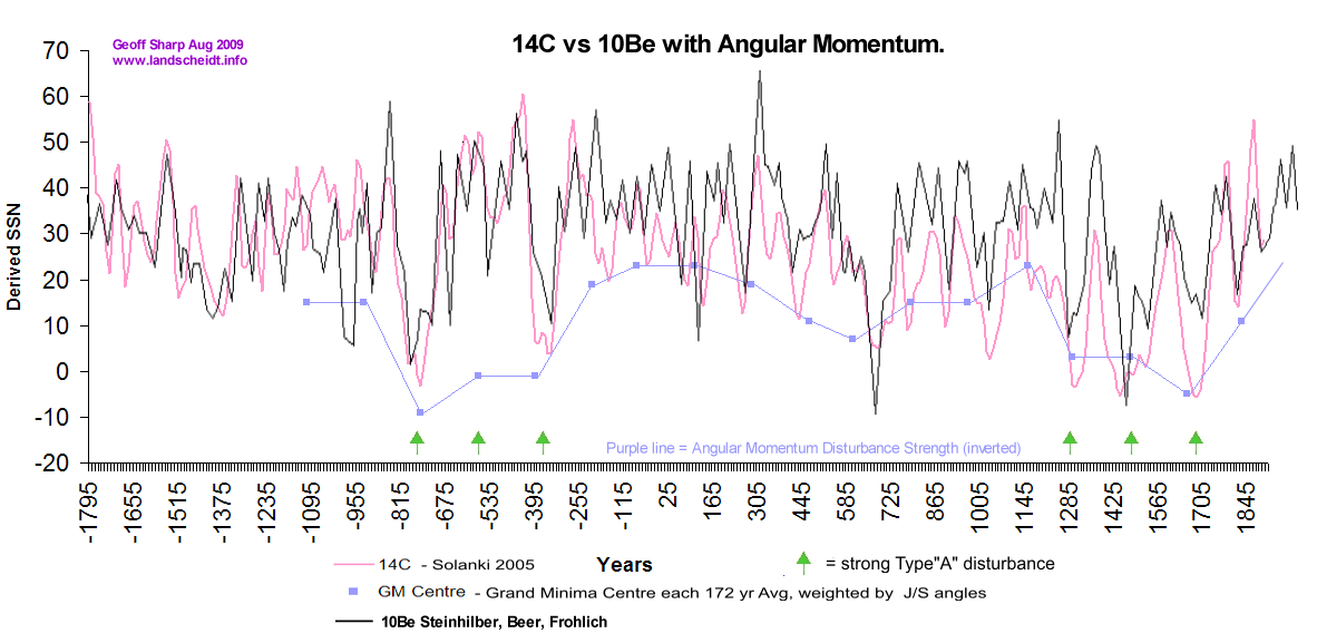
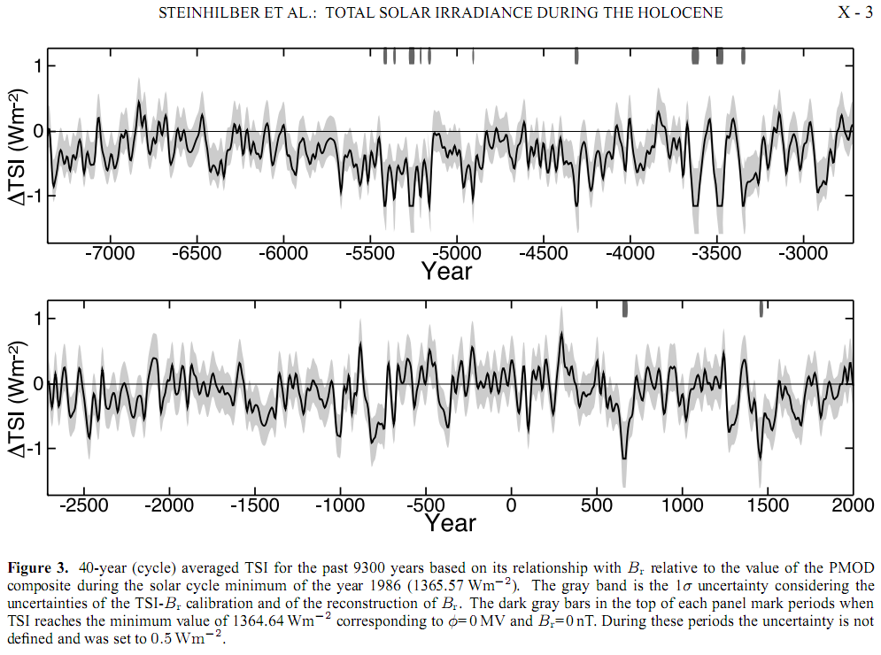
These disturbances always line up with periods of solar downturn. The Solanki/Steinhilber data shows regular solar downturns that vary in intensity, by observing the shapes of the disturbances that align with these downturns we are able to see a pattern that is repeatable. An example of this is the regular appearance of strong Type “A” disturbance occurring at times of severe grand minima. Weak Type “B” disturbance always is associated with very minor grand minima. There is no indication of this pattern not following suit except in the rare occasion of strong Type “A” disturbance not fully firing when not meeting the “Wilson’s Law” test. This test states that for a disturbance to fire the Jupiter/Saturn opposition or conjunction must happen before cycle max. This has been tested over the Sunspot numbers but is not available for accurate testing beyond that as the cycle max is not known. 1830 and -530 are examples of this phenomena.

Described in previous articles Type “A” is nearly always stronger than Type “B” disturbances. Type “A” affecting the inner loop of the Sun’s path around the SSB and Type “B” affecting the outer loop. The Sun’s velocity is 100% higher when traveling the outer loop.

By matching the disturbance patterns with solar downturn strength I gave each disturbance a score. Disturbance’s that align with deep grand minima (on a constant basis throughout history) get the highest score and so on.

On the solar proxy graph at the top of this article I have recorded the strength of each disturbance group that comes along every 172 years average. This was achieved by scoring each individual disturbance and summing. The individual disturbances can be viewed at http://www.landscheidt.info/?q=node/5 and http://www.landscheidt.info/?q=node/1

–
–
–

 

This table is a result of that process. The “Count” column being the sum of the individual disturbances for each 172 year centre. To plot this trend on the Solanki data it needs to be scaled and inverted. For the scale I tried to approximate the Solanki derived sunspot number and use a conversion process to do this within a set scale. For every increment of the “Count” I have associated it with 4 Solanki sunspots as seen on his graph. This gives a reliable method and displays the trend accurately. Once the conversion was done the data was entered into the Solanki spreadsheet.

Although the counting process is subject to the eye of the observer resulting in perhaps a slightly different Count, the overall trend will still be evident and should not vary greatly from my analysis. Future Counting could be performed more accurately by measuring the precise angles of the Jovians during individual disturbances and rating them according to a set scale. The ideal time to measure the angles is when Jupiter and Saturn are in opposition (measuring Neptune & Uranus angle in respect to Jupiter) for type “A” and when Jupiter and Saturn are at conjunction for type “B” disturbances. The position of the hump at disturbance is a direct result of the timing of Neptune and Uranus in respect to Jupiter.

Below is a table showing the conversion process.

 

The spreadsheets is available from http://www.landscheidt.info/images/solanki_sharp.xls

 

 

New 10Be Study Confirms 14C Record.

The Carbon 14 record (INTCAL98) used as a solar proxy as used by Solanki and Usoskin is sometimes called into doubt. There have been attempts to cross check the results using  beryllium 10 (10Be) comparing running means over different time periods. But now we have a new report that produces 9300 years of 10Be data that can be compared with the 14C record. Initial results show a very promising match up.

The new report which can be found here  http://www.leif.org/EOS/Holocene-TSI.pdf shows one graph in particular that can be used to cross check the 14C record. Click on graphs for a full size view.

The comparison graph is a first pass and should be extended the full 9300 years and if possible the new data needs to be merged with Solanki’s data in a spreadsheet. My method of comparison as follows: The 14C data is taken directly from the Solanki data and graphed via excel spreadsheet. The Steinhilber graph saved from the original document is traced onto a transparent gif image layer and saved then overlaid onto the original Solanki graph. The Steinhilber overlay is then rescaled for X & Y coordinates to match the original Solanki scale.

There are a few anomalies between the 2 data sets but overall a very good match is found. The 14C record is now confirmed with perhaps some minor anomalies but some confidence is expected. The planetary line ups with their disturbance to Angular Momentum that cause Grand Minima are now validated by another independent source.

Vale Carl Smith.

Wednesday 24th June 2009 at 3:35pm at Gold Coast Hospital (Wed gold coast time) Carl Smith lost his battle with cancer. Its a very sad day for his family, friends, associates and myself. I didnt have a lot to do with Carl and respected his wish of not interrupting the remaining quality time that was left for him.

Carl will be sadly missed and I know a lot of people have spoken highly of him. Carl was the originator of this website and only gave up the day to day running when he learned of his severe illness. He will be remembered for perhaps making the biggest discovery in the Planetary Theory Arena, Jose and Landscheidt were in the ballpark but Carl nailed it with his Angular Momentum graph that today allows us to predict solar activity and Grand Minimum down to the solar cycle.

I will continue to progress Carl’s work , he was a great man.

May I pass on sincere condolences from us all to the Smith Family.

Geoff Sharp.

UPDATE:25 july 2009

Carl’s brother Dave is keen to ensure that Carl’s work wont be wasted. I personally wont let that happen and consider myself with a new life’s work.

Dave has kindly donated a new domain and webspace to further this cause which will be run in conjunction with the original landsheidt auditblogs site.

The new site will be a showcase for Carl’s discovery and the further work I intend to do on the same topic. The site has all the bells and whistles and I encourage all to register.

The new site can be found here: http://www.landscheidt.info

New Angular Momentum Graph.

Its been a long time coming, but this graph is an easier way to appreciate the effect the outer planets have on our Sun. This is the same information Carl used in his now famous graph, but instead of a sine wave we have the absolute power shown in a conventional form. Angular momentum can be measured in different ways leading to confusion. Now we have a reliable power guide directed at the Sun from the Jovian planets.

Source: Carl’s JPL data assuming 2E+47 as a zero point and inverting all points below.

This next graph shows the sunspot cycle superimposed on the angular momentum strength…showing strong correlations. Notice how after a sudden slowdown the high angular momentum peaks are not fully utilized.

UPDATE 11/05/09:
The same graph but with the solar orbital velocity as it orbits the SSB overlaid. This shows the connection between Angular Momentum and the fluctuating speed of the Sun as it orbits the solar system barycenter, this orbit path being controlled by the outer planets. Conservation of angular momentum has consequences.

Below: This time I have compared the Sun’s velocity with the typical AM graph as per Carl….the altered velocity obvious at 1650, 1830 and 2010 which also correspond with radical Solar path changes caused by the outer planets. The Sun’s orbit speed is surprisingly slow and goes from around 30 km/h up to around 60 km/h (100% increase) when Angular Momentum is at its highest. This still allows the Sun to move over 1.5 million km from the SSB over 5 years. Note when the two lines diverge there is a corresponding slow down in solar activity.

This graph showing the velocity of the Sun is a product of Angular Momentum (red line = velocity). Interestingly velocity can exceed AM and also not use the full potential of AM. A conservation is required? Is there another force involved that modulates the usage of AM?

Now the question is, are there any other consequences, is the changing velocity also changing the rotation speed of the Sun as well. I have been searching for solar rotation rates but it seems we are unable to record this presently, there are no fixed points on the surface of the Sun which has a highly movable outer layer. The idea of a solar rotation change due to the planets is highly speculative, but until we can get an accurate measurement of solar rotation it cant be ruled out. If we could record the solar rotation accurately this discussion would be over…but we CAN record the rotation rate of Earth, and I postulate on the following with some brain food…… The Earth’s rotation rate is calculated by recording the Length of Day which shows our longest days (slower speed) are always in January. Theories suggest this is because of weather patterns that always occur in January but it also coincides with our planets fastest velocity which shows a very regular pattern each January.

Interesting pattern similar to the Jovian orbits…expecting earths orbit to follow the same trend.

Length of day graph from USNO showing the yearly rotation speed pattern of our planet. The slowest days are in January each year, which coincides with our closest approach to the Sun in our slightly elliptical orbit.

Which Point do the Jovian Planets Orbit?

This is an intriguing question, I have read many different opinions but nothing to clearly substantiate their claims. Others in the Scientific arena when pressed are afraid to give an answer. Checking the JPL data which is an ephemeris produced by the Jet Propulsion Laboratory shows that Jupiter certainly doesn’t orbit around the SSB (although at first because of an error I made, it looked as if it did) and probably orbits around the Jupiter/Sun barycenter. After checking the Jupiter/Sun distances (which I will refer to as the radius vector which is quite different from the semi-major axis) through JPL it became obvious there was a substantial variance each orbit that was measured each time in the same place. Originally I saw this as an opportunity to look for a solid link between Angular Momentum and the Solar modulation re the planets, but soon discovered Jupiter and all the other planets have a modulating Perihelion/Aphelion distance. The quest was on the find out why and involved many weeks searching for any data I could find. Others on this site got involved and I even emailed an Astronomer but to no avail, very sparse detail available. Dr Svalgaard suggested it was a result of planetary perturbations and while correct his understanding was also far from complete. Below is an account of the progress along with what I think is the complete answer to what perturbs Jupiter and how.

————————————————————————————————————————————————————
My research shows the Jupiter/Sun distance varies on average 300,000 km each orbit of Jupiter. Check graphic above.
The Earth is seen to orbit the Sun directly. If we use NASA’s JPL data it shows the Earth/Sun distance is varying by 0.0001AU per year (approx 15000 km). The AU measure is the average distance between the Sun and Earth. If we measure The Earth to SSB (solar system barycenter) distance it shows a much larger variance.
What I have done is measure the Jupiter/Sun distance at exactly the same point in the elliptical orbit of Jupiter each 4331.572 days, this should isolate any aphelion/perihelion changes. I also measured the Jupiter/SSB distances.

As can be seen in the first graphic there is a large variance each orbit between BOTH measurements (Sun & SSB). This makes it hard to pinpoint any point of orbit, although the variances seem smaller on average with the Jupiter/Sun data. I also compared the Heliocentric longitude (angle away from Sun) and found each Jupiter/Sun reading had an angle of 359 deg, but the solar position at perihelion does return very closely to the same position each orbit.

The above graph was made from reliable data by blogger JimP (thanks for the spreadsheet). Once blown up it shows some remarkable detail. It shows the Perihelion distance (closest point) for each Jupiter orbit over 400 years. There is a definite pattern, what causes this modulation? The movement between the closest and furthest perihelion is 1.2 million km’s , the Sun is capable of moving 1.5 million km’s from the barycenter, Neptune’s radius vector moves by 1.4 million km. Importantly the corresponding movement at the other end (aphelion) is the same value on each orbit but in the opposite direction, if one end shortens the other end lengthens.

Jupiter/Sun distances 1600-2020 with Jup/Sat conjuncture, Jup/Sat opposition and Jup/Sat quadrature (square) positions plotted for every third occurrence. Note the phase change around 1880. If the Variance in distance is caused by angular momentum J/S conjunction & J/S opposition both produce high angular momentum. Regular reader lgl and myself suspect the other Jovians need to come into the equation, but what is needed is a new method of displaying angular momentum other than Carl’s graph. A total strength with both J/S conjuncture and J/S opposition shown as high points instead of a sine wave is required, manipulation of the current JPL data via a spreadsheet can do it. Update: There is a new article covering this.

Saturn/Sun distance showing the same 60 yr pattern as Jupiter. After 1880 they are in unison with Jupiter but not before. There is a reason for these fluctuations but I have not found any literature on this phenomena.

UPDATE 13/05/09:

This diagram has been adapted from “Linkages between solar activity, climate predictability and water resource development” Alexander et al. Bailey has been criticized for claiming the Sun-Earth distance varies by the Sun-SSB distance, although not correct there is a fluctuation caused in the same manner as per Jupiter but to a smaller degree….0.0001 AU.

UPDATE 27/05/09: Here is another suggestion Dr. Svalgaard has provided to explain the modulating Jupiter Perihelion.

“The general principle is that to change the orbit, you have to apply a force along the orbit, so Saturn’s effect is largest when it is ‘to the side’ (approximately quadrature I think the astrological term is), rather than in conjunction. All of this has been understood for 250 years, and there are no other forces involved. Saturn doesn’t ‘push’ (gravity is attractive, not repulsive). And the Sun is not ‘dragging’: the force is always along the line connecting two bodies.
To recapitulate how Kepler’s second law works: To move an orbit out a bit (increase perihelion distance if you are near perihelion), you apply a force along the orbit in the same direction as the movement of the planet, e.g. by Saturn being ahead of Jupiter. That force produces a ‘delta-v’ (google it), which ‘lifts’ the orbit a bit out of the gravitational well, to another (higher) orbit, where it actually moves slower than before. Because of the periodic movements, the lifting is counteracted over time by a similar but oppositely directed movement, so that the semi-axis stays constant. This takes a couple of orbits to accumulate, so you have to consider the integrated effects over many years.”

There is substantial merit in Dr. Svalgaard’s rejigged explanation, but there still remains some pertinent questions. The explanation works well for perturbations occurring in the 1/2 to 3/4 region before Perihelion, but perhaps not so well in others. Dr. Svalgaard explains its a matter of the smaller background oscillations that make it hard to track the source of the perturbation. This is plausible but maybe a little weak and may be the reason it is near impossible to find any reliable data on this topic via the web. In particular I have questions why the “force along the orbit” fails to work when Jupiter approaches Perihelion and actually looks to have an opposite effect. Remember, when Jupiter & Saturn are in conjunction the Perihelion distance is at its shortest, but as you can see in the following diagrams the substantial pull along the orbit fails to elevate Jupiter’s orbit to a higher state.

The red dots signifies Perihelion in this 1762 example:

I wanted to see the perturbation affects plotted with successive orbits to see how the planets contribute to Jupiter’s orbit changes. Although fairly easy when you know a couple of tricks (thanks to Dr. Svalgaard) this task took me many days. I plotted the JPL data into excel and once the orbit was expanded to a size too big to display here it was easy to see each individual orbit. I was lucky with my data selection because it included a very strong perturbation of the 1987 Perihelion. The orbit has Jupiter doing a fly past Saturn, Uranus and Neptune before Perihelion which manages to take it away from its more normal path by 6 million kilometers. Once Jupiter passes all 3 planets its orbit is dramatically “braked” which brings it back into line around Perihelion, but still manages a very long perihelion distance. This is a good example of the perturbation theory in practice.

The corresponding planetary view shows the relative positions of planets which line up with the above average perturbation.

So do we have a situation where the perturbation theory works in some parts of the orbit only? Could other forces be overriding this perturbation? The orbit changing mechanics have been described as speeding up the planets velocity (I have serious reservations that this occurs) which raises it up the gravity well to a higher orbit before settling into a slower overall velocity.
————————————————————————————————–
UPDATE:After much research I think I finally have the cause for Jupiter’s Perihelion distance modulation….and it surprising how little is known or published in this area. The above example is not worded very well and leads you to think an acceleration lifts the orbit higher then slows the velocity (that’s at least how I read it), from what I now understand it actually happens in reverse…the acceleration moves the orbit closer (following Kelper’s 2nd Law) but then unlike a rocket using boost, Jupiter is then immediately subjected to deceleration from Saturn’s gravity which slows velocity in turn lengthening the radius vector or raising Jupiter to a higher orbit. As Jupiter moves further away from Saturn the Sun takes over and reins in its sibling and waits for the next perturbation. So now it becomes obvious, and completely explains why a Jupiter/Saturn conjunction causes a short Perihelion, Jupiter is always in acceleration mode during this lineup which causes it to move closer and the plotted orbit agrees. Also of note, Neptune and Uranus also help out and can be strong when together as we see elsewhere on this site.

The orbit spreadsheet is able here: http://users.beagle.com.au/geoffsharp/jup_orbit1940-2009.xls

Spin–Orbit Coupling Between the Sun & Jovian Planets.

This Paper by I. R. G. Wilson, B. D. Carter, and I. A. Waite is now available free onliine. http://www.publish.csiro.au/?act=view_file&file_id=AS06018.pdf

Abstract:We present evidence to show that changes in the Sun’s equatorial
rotation rate are synchronized with changes in its orbital motion about the
barycentre of the Solar System.We propose that this synchronization is
indicative of a spin–orbit coupling mechanism operating between the
Jovian planets and the Sun. However, we are unable to suggest a plausible
underlying physical cause for the coupling. Some researchers have proposed
that it is the period of the meridional flow in the convective zone of the Sun
that controls both the duration and strength of the Solar cycle.We postulate
that the overall period of the meridional flow is set by the level of disruption
to the flow that is caused by changes in Sun’s equatorial rotation speed.
Based on our claim that changes in the Sun’s equatorial rotation rate
are synchronized with changes in the Sun’s orbital motion about the
barycentre, we propose that the mean period for the Sun’s meridional flow
is set by a Synodic resonance between the flow period (?22.3 yr), the overall
178.7-yr repetition period for the solar orbital motion, and the
19.86-yr synodic period of Jupiter and Saturn.
——————————————————————————————–

Some very interesting sections of this paper discuss changes in angular momentum and solar equatorial rotation change. I would like to see more work in this area, as there is scant amount of detail available on my searching. There must be someone working on comparing current solar differential rotation with other periods?

In another section the paper acknowledges the work done by Fairbridge & Shirley 1987 in using all of the Jovian planets to calculate angular momentum but unfortunately dont include Neptune & Uranus any further. I believe Fairbridge & Shirley were SO close in 1987 but failed to see the absolute importance of Neptune & Uranus…they had a graph like Carl’s but didnt cross check it against the planetary line ups. Incredible that they went so far but didnt go the extra step. Its now some 22 years later.

But the most important discovery by Wilson et al in this paper in my view, is their “phase locking” theory. Grand Minima type events (SSN less than 80) have happened in the past when the conjunction of Jupiter & Saturn happens before that cycle’s maximum, implying a mechanism of catch up, keeping the Jupiter/Saturn sysygies in line with solar cycles. I refer to this in other articles as “Wilson’s Law”. If SC24 peaks after March 2011 it will fit that criteria as well as SC25 if it peaks after Nov 2020. This phenomenon has always happened at or just after the “camel hump” disturbance on Carl’s graph, and begs the question: Does this phenomenon happen as a result of the major disturbance to the angular momentum or is that just coincidence? To test this I might plot all the sysygies and cycle max’s on Carl’s Graph.

UPDATE: below is a graph showing J+S sysygies with sunspot peaks, Note: pre 1700 solar cycle maxima is derived geomagnetic aa proxy figures, click on the graph for a larger image.

Ian’s work has answered some of my questions and explains why 1830 didnt invoke further Grand Minimum action, also why 1880 (SC12) was low during higher angular momentum, Its obvious if the aa records are correct that we have a higher frequency of early J+S sysygies with the higher angular momentum caused by N+U.
Black dots are J+S together, Blue dots J+S opposed, and Red dots are solar cycle maxima…..reduced solar activity occurs if we get a black or blue dot in between cycle minimum and before cycle maximum

Geoff.

Ian Wilson's Theory on the Planetary Influence on Grand Minima.

Ian Wilson, highly respected Australian scientist working in the area of planetary influence on solar activity has provided us with his paper outlining his theory on some possible drivers of solar grand minima. This area of science seems to be on the fringe where no matter what funds are available no real knowledge can claim with total confidence how the next cycle will pan out, let alone when the next Maunder type minimum might happen, its an open arena waiting for a credible explanation.
Landscheidt Cycles welcomes Ian’s paper which can be accessed through this link:http://plasmaresources.com/ozwx/wilson/Syzygy.pdf
Below is a graph from Ian’s paper showing the heliocentric latitude of Venus (solid line) and the mean distance of Jupiter from the Sun in astronomical units (dashed line), we welcome constructive debate.

Landsheidt Blog Admin Change

Due to my ongoing ill health while fighting a very aggressive cancer, I simply do not have time to do any justice to the work that needs to be done in furthering what Dr Landsheidt and many others were/are exploring with regards to Solar Activity Cycles and Extraterrestrial Influences on the Earth’s Climate.

As a consequence I put out an appeal for blog Administration assistance, and I am both thankful and happy to say that Geoff Sharp now has full Admin privileges assigned for this blog, and I am henceforth handing over the the day to day running of the blog into his more than capable hands.

Geoff has a range of editorial and graphic design skills that should aid him in revitalizing the look and feel of the blog over time while also expanding it’s scope to reach a broader audience, and I am looking forward with interest to see where he takes it.

I would also like to take this opportunity to extend a special thank-you to contributer Ulric Lyons for also putting up his hand and trying to get registered to take up Admin duties after I made my health issues public – I am sure Ulric will have more to contribute concerning his planetary position material when ready to do so, and encourage him to keep working at it.

Another well deserved thank-you goes to Auditblogs founder John A for not only providing the free Auditblogs blog hosting service that made this blog possible in the first place, but in also extending his valuable time by helping get Auditblogs registration issues sorted out – anyone who wants to help John A offset his out-of-pocket costs in providing this free service can do so using the donation box at Auditblogs.

I wish Geoff all the best as the new Admin for the Landscheidt Cycles Research blog.

Carl.

Health Issues

Just a quick note to let you all know that after a long period of illness I have been diagnosed as having a neuroendocrine cancer of the bladder that has metastasized into the lymph nodes in my pelvis and the bones in my hips and spine.

This means I will be quite busy trying to tilt the odds more in my favour, and will not be able to contribute much here for the forseeable future. 

I feel that there is important work to be done here, and I am quite prepared to grant admin privileges to one or more of the regular contributers to further things, as I am too preoccupied to continue with it myself  – just let me know via email and we can work it out.  

THE SUNSPOT CYCLE AND C24

Guest post by Ulric Lyons

THEORY:

1) The SS cycle is caused by heliocentric syzygies of Jupiter, Earth and Venus. The average time between the tightest alignments over 100yrs. is 11.086yrs. The alignments alternate between E opposite V in line with J in one cycle, and E and V together in line with J, in the next cycle, in sync with the magnetic reversal of the Sun.

2) The position of the center of each maximum moves relative to the tightest alignments, earlier if the cycle is augmented, and later if the cycle is diminished. C3 to C8 is a good example of this.

3) The amplitude of each cycle is governed by a) the relative positions of Jupiter, Saturn and Uranus, and, b) the positions of E and V in relation to J, S and U.

4) The peaks on every cycle are largely due to syzygies of E+V, J+E, J+V and stelliums of all three. Hence the SS record can be seen to be a recording of these alignments, which usually can be correlated to stronger monthly temperature anomalies.

PROJECTIONS:

Maximum center for C24 estimated at 1yr. before the alignment center = early 2013. It will be augmented from 2010 to 2013, with peaks above C23, strongly in 2010, with August and October being likely dates for large solar flares.

The relative positions of U,S,J,E and V start to fall into diminished configurations from late 2013/early 2014, leading to a lower sunspot count in second half of the cycle. This will be accompanied by increasingly lower global temperatures from 2014 to 2020. A good measure of this can be seen by looking back 179yrs on the CET series:
http://www.metoffice.gov.uk/research/hadleycentre/CR_data/Daily/HadCET_act.txt
ie., lookat years 1835 to 1841 for 2014 to 2020.

Smoke & Pollen

Just a quick note to let visitors to this site know that due to my state of health I will not be able to contribute much here until further notice.

During the late-winter early-spring period every year I suffer pollen allergies that effect my sinuses and lungs, and my ability to focus and concentrate my attention on things, however this year the effects are being exacerbated by the ongoing smoke from bushfires for the last month, many of which are controlled burns to reduce unusually heavy fuel loads before the hot weather arrives later in the year

My health has become quite run down by this unrelenting assault on my immune system.

All my research projects are now on hold until I can breathe more easily and regain my ability for sustained concentration – my public participation in things will be limited to occasional posts on various forums, as I think I can manage that some of the time – however I may also need to let that go for a bit if my situation deteriorates further.

UPDATE 2007-08-14:

Was looking at the new BoM Brisbane doppler radar viewer and was quite interested to see the smoke from the fires clearly imaged in the area near the radar site!

See screen capture below (colour enhanced to show detail):

Note the large coloured areas showing the smoke near the radar site, and the red dot below the first ‘e’ in Beenleigh and another above the ‘o’ in Logan showing the positions of active fires with smoke rising fast above them!

Below is the latest visible light satpic so you can see the scattered cumulous clouds also depicted as small smudges on the radar for comparision:

Due to the time it takes the satellite to scan the Earth, the time of the satpic is about 0150 utc, about 22 minutes before the radar capture.

The GFS computer model is being optimistic about 50+mm of rain here next week:

Let’s hope it comes off, drowns the fires, and clears the pollens from the air – but I will not hold my breath waiting – GFS often starts bullish then backs off later – we have had no rain to speak of here for about 2 months now!

Meanwhile, I’m still half-dead from smoke and pollen here!!!

My location is just SW of the lower left corner of the marker for Miami in the radar image and the air is think with a smoke haze … um … I mean thick with smoke haze 😦 … I have a headache and my eyes are watering while I’m trying to write this …

UPDATE 2007-08-18:

Relief in sight at last!

GFS is getting more bullish as the days go by:

BoM Satellite image shows things are looking up:

Sea Surface Temperature anomoly is looking good for rain to develop in coastal SE Qld with warm area along coast:

And the Global SST anomoly shows La Nina is probably nearly here as well with a cool tongue extending west across the equatorial Pacific from Sth America, meaning a good wet season is likely here in the coming months:

Looking forward to some decent rain to clear out the smoke and pollen so I can breathe freely again and think more clearly, as there are things I wish to get on with!

UPDATE 2007-08-21

Rain … lots of it!

We have had several inches over the last couple of days, a 50 knot East Coast Low [sub-tropical cyclone] has developed off the coast, the bushfires have been washed out, and the pollen has all blown away!

I am starting to breathe again, and should be feeling much more healthy within a few days as my body recovers from the smoke and pollen onslaught … what more can I say? 🙂

Linkages between solar activity, climate predictability and water resource development

An interesting new paper may point to a way of improving on Dr Landscheidt’s methods:

Linkages between solar activity, climate predictability and water resource development
by W J R Alexander, F Bailey, D B Bredenkamp, A van der Merwe and N Willemse

Abstract:

This study is based on the numerical analysis of the properties of routinely observed hydrometeorological data which in South Africa alone is collected at a rate of more than half a million station days per year, with some records approaching 100 continuous years in length. The analysis of this data demonstrates an unequivocal synchronous linkage between these processes in South Africa and elsewhere, and solar activity. This confirms observations and reports by others in many countries during the past 150 years. It is also shown with a high degree of assurance that there is a synchronous linkage between the statistically significant, 21-year periodicity in these processes and the acceleration and deceleration of the sun as it moves through galactic space. Despite a diligent search, no evidence could be found of trends in the data that could be attributed to human activities. It is essential that this information be accommodated in water resource development and operation procedures in the years ahead.

I will expand on this as soon as I find the time.

Open Comments Thread

As an experiment, I thought I’d set up an open comments thread for your suggestions or general comments or whatever, and which may include offtopic material as well, so we shall see what happens …. over to you!

Note: the problem with the spam filter that was stopping some posting here has been fixed -however it also told a lie by telling people their comments were awaiting moderation, but it did not put them in the moderation cue, so for anyone that did encounter this problem, unfortunately the stopped comments are nowhere to be found. I apologise for any inconvenience, and plead that being new to blog admin, I am still learning how the various blog controls operate and interact with each other!

If anyone has any further problems, contact me by emailing:

carls AT qldnet DOT com DOT au

– written to avoid spam – most of you know what to do!

Newcomers: copy the email address above and paste it in the To: field of your email program, replace the AT part with @ and both cases of DOT with . and remove all blank spaces.

“Landscheidt is an astrologer”

I knew this issue would probably arise, so I might as well deal with it now.

I am quite aware that Dr Landscheidt studied astrology, as did Nicolas Copernicus, Johannes Kepler, Tycho Brahe, Issac Newton, and many other luminaries of science, so I would say that puts him in some pretty good company!

The fact of the matter is that I have also studied astrology – I think it goes with the territory of having intense curiousity about the universe and an open mind – but having done so I do not buy into the popularist and fatalist versions, but concede that there may indeed be “something in it”, especially in the sense that planetary cycles have been shown to effect the behaviour of the Sun, and in doing so the climate on the Earth.

Let me say right up front that I am not going to be investigating Dr Landscheidt’s more esoteric astrological material here on this blog, but rather will in the main be focussing on his solar cycle work which does have a physical basis, and which can be tested and verified or falsified, so therefore qualifies as science, no matter what some may think of his other interests.

As I have seen many of Dr Landscheidt’s climate predictions come to pass, along with a few misses, I consider his predictive material for solar activity and climate does have some merit, and is therefore worthy of further investigation.

Edit Note: Steve M deleted the offending comment on ClimateAudit the quote above was originally from, so I have removed the link and the comment from here, and shortened the reference in the title to just a generic version of the key phrase.

New Little Ice Age Instead of Global Warming?

To follow up on my previous post, I thought it might be good to examine the paper:
New Little Ice Age Instead of Global Warming?

Abstract: Analysis of the sun’s varying activity in the last two millennia indicates that contrary to the IPCC’s speculation about man-made global warming as high as 5.8° C within the next hundred years, a long period of cool climate with its coldest phase around 2030 is to be expected. It is shown that minima in the 80 to 90-year Gleissberg cycle of solar activity, coinciding with periods of cool climate on Earth, are consistently linked to an 83-year cycle in the change of the rotary force driving the sun’s oscillatory motion about the centre of mass of the solar system. As the future course of this cycle and its amplitudes can be computed, it can be seen that the Gleissberg minimum around 2030 and another one around 2200 will be of the Maunder minimum type accompanied by severe cooling on Earth. This forecast should prove skillful as other long-range forecasts of climate phenomena, based on cycles in the sun’s orbital motion, have turned out correct as for instance the prediction of the last three El Niños years before the respective event.

If Dr. Landscheidt is correct about this, we are about to enter an extended period of much reduced solar activity and therefore an extended period of global cooling, which will offer the first real world test of the IPCC’s CO2 forced global warming claims. On the downside of this, a return to climate conditions not experienced since about 1670 by the year 2030 will bring much hardship to millions, as many of the world’s foodbowls fail due to extreme cold, while demand for fossil fuels will increase just so people can survive the extreme cold in higher latitudes.

Unfortunately, the current obsession with global warming pseudoscience combined with hefty increases in the price of carbon use being planned and/or implemented in various countries means that very few will be prepared for the sudden significant downturn in temperatures likely to begin manifesting during the next few years, and as is so often the case, the poor will be the ones that suffer most due to the incompetence of certain prominent scientists prepared to over state the soundness of their science on the basis of a prejudicial belief, combined with a well orchestrated media campaign that has convinced much of the public and policymakers of the need to make huge sacrifices in order to ‘save the planet’ from a human induced fever that in fact probably only exists in the minds of the ‘true believers’.

Dr Landscheidt’s Solar Cycle 24 Prediction

As we approach Solar minimum, I thought it might be worthwhile to examine what Dr Landscheidt had to say about future of Solar Cycles and how things look for upcoming solar cycle 24.

Perhaps the best approach is to take a close look at this definitive paper:

EXTREMA IN SUNSPOT CYCLE LINKED TO SUN’S MOTION
THEODOR LANDSCHEIDT
(Received 21 May 1999; accepted 13 September 1999)
Abstract.

Partitions of 178.8-year intervals between instances of retrograde motion in the Sun’s oscillation about the center of mass of the solar system seem to provide synchronization points for the timing of minima and maxima in the 11 -year sunspot cycle. In the investigated period 1632-1990, the statistical significance of the relationship goes beyond the level P = 0.001. The extrapolation of the observed pattern points to sunspot maxima around 2000.6 and 2011.8. If a further connection with long-range variations in sunspot intensity proves reliable, four to five weak sunspot cycles (R < 80) are to be expected after cycle 23 with medium strength (R ~ 100).

The part I bolded is a most interesting prediction of upcoming solar activity.

As we have not yet reached solar minimum, and no high latitude cycle 24 spots have yet appeared, we may still be 12 to 18 months from minimum if recent cycles are anything to go by, and I venture a speculation that if no cycle 24 spots appear in the very near future then perhaps Dr Landscheidt should have also mentioned the other possible date of the upcoming solar max using his methods, 2013.6 (see details of his methods in the paper), which if it turns out to be true means a very long cycle which could indicate a very low sunspot max.

Examination of Dr. Landscheidt’s Work

My intent is to work though parts of several of Dr. Landscheidt’s papers both to verify and if possible update some of his findings. My current thoughts are to start with some of his earlier work, as this is where he lays out his methods in the most detail.

This process will take some time as I have a life elsewhere, and I am a bit slow doing things anyway, so do not expect fast progress in this. Update 2007-Jun-01: As I tend to chop and change a bit, and am somewhat addicted to editing what I’ve written anyway, I may edit earlier posts at times, and will hopefully remember to indicate what I’ve changed!

Dr Theodor Landscheidt & Solar Cycle Research

Over several decades until he passed away on May 20, 2004, Dr Theodor Landscheidt wrote extensively on the torque cycle of the planets in their orbits about the Sun causing a transference of angular momentum back and forth between the Sun and the planets in a quite predictable manner, and showed how it correlates quite well with both solar activity cycles and some aspects of the Earth’s climate.

Rather than rehash what is already written elsewhere, here are a couple of paragraphs quoted from the webpage So, What’s New In Our Universe? by Gary Sharp: